Copyright ©
This work is licensed by a Creative Commons license .
First printing, February 2022
First, this thesis is dedicated to my family. We are a small family: my parents, my grandparents and my uncles and aunt. Specially, to my mother, who has never failed to encourage me to follow what I like to study, also for her constancy in response to my chaos. Also, specially to my father, from whom I got the passion for photography and computer science. Knowing this one could understand better this thesis. To my paternal grandparents who are no longer with us. To my maternal grandmother who always has good advice. Recently, she said to my mother: "the kid has studied enough; since you send it to kindergarten with 3 years, he hasn’t stopped", referring to this thesis!
To my friends, beginning with Anna, who is my flatmate and my partner; and who has supported me during these final thesis months. To other friends from the high school, both neighborhoods I grew up and those friends from the faculty, also. To other colleagues with whom I have shared the fight for a better university model, and now we share other fights, to my comrades!
To the Department of Electronics and Biomedical Engineering of Universitat de Barcelona, to all its members. Specially, to Dr. A. Cornet for being a nice host at the department. Specially, to Dr. A. Herms, to encourage me to pursue the thesis in this department and to contact Dr. J. D. Prades, director of this thesis. Also, to other colleagues from the MIND research group i from the Laboratory from ’the \(\mathrm{0}\) floor’: to Dr. C. Fàbrega, to Dr. O. Casals, and many others!
To Dr. J. D. Prades himself, for the opportunity by accepting this thesis proposal, and embrace the idea I presented, leading to the creation of ColorSensing. To the ColorSensing team, begining with María Eugenia Martín-Hidalgo, co-funder and CEO of ColorSensing. Without forgetting, all the other teammates: to Josep Maria, to Hanna, to Dani, to María, to Ferran and to Míriam (Dr. M. Marchena). But also, to the former teammates: to Peter, to Oriol (Dr. O. Cusola), to Arnau, to Carles, to Pablo, to Gerard, to Hamid and to David. Thank you very much all for this journey.
This thesis has been funded in part by the European Research Council under the FP7 and the H2020 programs, no. \(\mathrm{727297}\) and no. \(\mathrm{957527}\). Also, by the Eurostarts program with the Agreement no. \(\mathrm{11453}\). Additional funding sources have been: AGAUR - PRODUCTE (\(\mathrm{2016-PROD-00036}\)), BBVA Leonardo, and the ICREA Academia program.
Aquesta tesi va dedicada en primera instància a la meva família. Som una família petita: a mons pares, als meus avis i als meus tiets. Especialment, a ma mare, perquè mai a fallat en animar-me per perseguir el que m’agrada estudiar, també per la seva constància davant del meu desordre. Especialment també, al meu pare, per la seva passió amb la fotografia i la informàtica que des de petit m’ha inculcat, així hom pot entendre aquesta tesi molt millor. Als meus avis paterns que ja no estan. A la meva àvia materna que sempre té bons consells, i fa poc li va dir a ma mare: "si el nen ja ha estudiat prou, d’ençà que el vas portar amb tres anys (al col·legi) no ha parat d’estudiar", referint-se a aquesta tesi!
Als meus amics, començant per l’Anna, que és la meva companya de pis, i la meva parella; que m’ha recolzat durant aquests darrers mesos a casa mentre redactava la tesi. A tots aquells amics de l’institut, del barri, de la ’urba’ i de la facultat. També a aquelles companyes amb les quals hem compartit lluites a la universitat des de l’època d’estudi i ara seguim compartint altres espais polítics, els i les meves camarades.
Al Departament d’Enginyeria Electrònica i Biomèdica de la Universitat de Barcelona, a tots els seus membres. Especialment, al Dr. A. Cornet per la seva acollida al departament. Al Dr. A. Herms, per animar-me a fer la tesi al Departament i contactar al Dr. J. D. Prades, director d’aquesta tesi. També, a altres companyes i companys del MIND, el nostre grup de recerca, i del Laboratori ’de planta \(\mathrm{0}\)’: al Dr. C. Fàbrega, la Dra. O. Casals, i tots els altres!
Al mateix Dr. J. D. Prades, per l’oportunitat acceptant aquesta tesi, i acollir la idea que li vaig presentar fins al punt d’impulsar la creació de ColorSensing. A tot l’equip de ColorSensing, començant per la Maria Eugenia Martín-Hidalgo, cofundadora i CEO de ColorSensing. Però, per suposat, a la resta de l’equip: al Josep Maria, a la Hanna, al Dani, a la María, al Ferran i a la Míriam (Dra. M. Marchena). Però també als seus antics membres amb qui hem coincidit: al Peter, a l’Oriol (Dr. O. Cusola), a l’Arnau, al Carles, al Pablo, al Gerard, a l’Hamid i al David. Moltes gràcies a tots i totes per fer aquest viatge conjuntament.
Color-based sensors, where a material change its color from one color to another, and this is change is observed by a user who performs a manual reading, often offer qualitative solutions. These materials change their color in response to changes in a certain physical or chemical magnitude. We can find colorimetric indicators with several sensing targets, such as: temperature, humidity, environmental gases, etc. The common approach to quantify these sensors is to place ad hoc electronic components, e.g. a reader device.
With the rise of smartphone technology, this thesis builds around the possibility to automatically acquire a digital image of those sensors and then compute a quantitative measure is near. By leveraging this measuring process to the smartphones, we would avoid the use of ad hoc electronic components, thus reducing colorimetric application cost. However, there exists a challenge on how-to acquire the images of the colorimetric applications and how-to do it consistently, coping with the disparity of external factors affecting the measure, such as ambient light conditions or different camera modules.
In this thesis, we tackle the challenges to digitize and quantify colorimetric applications, such as colorimetric indicators. We make a proposal to use 2D barcodes, well-known computer vision patterns, as the base technology to overcome those challenges. Our research focused on four main challenges: (I) to capture barcodes on top of real-world challenging surfaces (bottles, food packages, etc.), which are the usual surfaces where colorimetric indicators are placed; (II) to define a new 2D barcode to embed colorimetric features in a back-compatible fashion; (III) to achieve image consistency when capturing images with smartphones by reviewing existent methods and proposing a new color correction method, based upon thin-plate splines mappings; and (IV) to demonstrate a specific application use case applied to a colorimetric indicator for sensing \(CO_2\) in the range of modified atmosphere packaging –MAP–, one of the common food-packaging standards.
Els sensors basats en color, normalment ofereixen solucions qualitatives, ja que en aquestes solucions un material canvia el seu color a un altre color, i aquest canvi de color és observat per un usuari que fa una mesura manual. Aquests materials canvien de color en resposta a un canvi en una magnitud física o química. Avui en dia, podem trobar indicadors colorimètrics que amb diferents objectius, per exemple: temperatura, humitat, gasos ambientals, etc. L’opció més comuna per quantitzar aquests sensors és l’ús d’electrònica addicional, és a dir, un lector.
Amb l’augment de la tecnologia dels telèfons intel·ligents, aquesta tesi explora les possibilitats d’automatitzar l’adquisició d’imatges digitals d’aquests sensors i després computar una mesura quantitativa és a prop. Desplaçant aquest procés de mesura als telèfons mòbils, evitem l’ús d’aquesta electrònica addicional, i així, es redueix el cost de l’aplicació colorimètrica. Tanmateix, existeixen reptes sobre com adquirir les imatges de les aplicacions colorimètriques i de com fer-ho de forma consistent, a causa de la disparitat de factors externs que afecten la mesura, com per exemple la llum ambient or les diferents càmeres utilitzades.
En aquesta tesi, encarem els reptes de digitalitzar i quantitzar aplicacions colorimètriques, com els indicadors colorimètrics. Fem la proposta d’utilitzar codis de barres en dues dimensions, que són coneguts patrons de visió per computador, com a base de la nostra tecnologia per superar aquests reptes. Hem enfocat la nostra recerca en quatre reptes principals: (I) capturar codis de barres sobre de superfícies del món real (ampolles, safates de menjar, etc.), que són les superfícies on usualment aquests indicadors colorimètrics estan situats; (II) definir un nou codi de barres en dues dimensions per encastar elements colorimètrics de forma retro-compatible; (III) aconseguir consistència en la captura d’imatges quan es capturen amb telèfons mòbils, revisant mètodes de correcció de color existents i proposant un nou mètode basat en transformacions geomètriques que utilitzen splines; i (IV) demostrar l’ús de la tecnologia en un cas específic aplicat a un indicador colorimètric per detectar \(CO_2\) en el rang per envasos amb atmosfera modificada –MAP–, un dels estàndards d’envasat alimentari.
The rise of the smartphone technology developed in parallel to the popularization of digital cameras enabled an easier access to photography devices to the people. Nowadays, modern smartphones have onboard digital cameras that can feature good color reproduction for imaging uses [1].
Alongside with this phenomenon, there has been a popularization of color-based solutions to detect biochemistry analytes [2]. Both phenomena are probable to be linked, since the first one eases the second. Scientists who want to pursue research to discover new or improve existent color-based analytics found themselves with better and better imaging tools, spending fewer and fewer resources.
Color-based sensing [2] is often preferred over electronic sensing [3] for three reasons: \(\mathrm{1}\)) the rapid detection of the analytes; \(\mathrm{2}\)) the high sensitivity; and \(\mathrm{3}\)) the high selectivity of colormetric sensors. Nevertheless, imaging acquisition on smartphone devices still presents some acquisition challenges, and how to overcome those challenges is still an open debate [4].
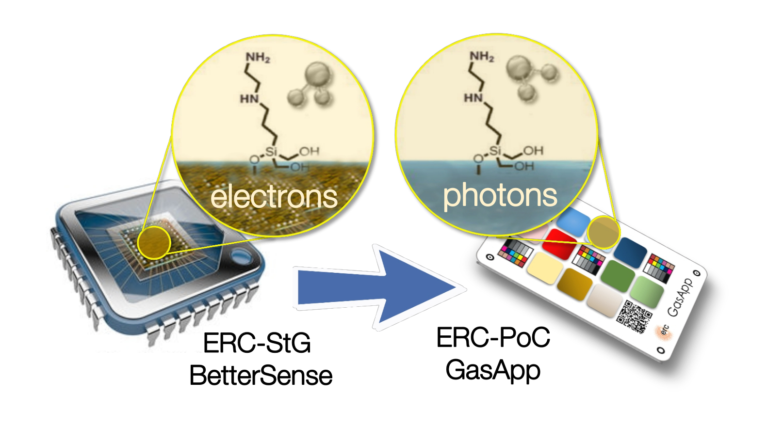
This is why, the ERC-StG BetterSense project (ERC n. 336917) was granted the extension ERC-PoC GasApp project (ERC n.727297). Bettersense aimed to address the high power consumption and the poor selectivity of electronic gas sensor technologies [5]. GasApp aimed to bring the capability to detect gases to smartphone technology, relying on color-based sensor technology [6].
The accumulated knowledge from BetterSense was translated into the GasApp project to create colorimetric indicators to sense target gases, the GasApp proposal is detailed in [fig:bettersense2gasapp]. Later on, the SnapGas project (Eurostars n. 11453) was also granted to carry on this research topic, and apply the new technology to other colorimetric indicators to sense environmental gases [7].
The GasApp proposal was based on changing from electronic devices to colorimetric indicators, thus leveraging the electronic components of the sensor readout to handheld smartphones. To do so, GasApp proposed a solution implementing an array with colorimetric indicators placed on top of a card-sized substrate to be captured by a smartphone device (see [fig:bettersense2gasapp]).
The design of this array of colorimetric indicators presented several challenges, such as: detecting and extracting the card and the desired region of interest (sensors), embedding one or more color charts and later perform color correction techniques to achieve adequate sensor readouts at any possible scenario a mobile phone could take a capture.
The research of this thesis started in this context, and the work here presented aims to tackle these problems and resolve them with an integral solution. Let us go deeper in some of these challenges to properly formulate our thesis proposal.
First, the fabrication of the color-based sensors presents a challenge itself. There exists is a common starting point in printed sensors technologies to use ink-jet printing as the first approach to the problem to fabricate a printed sensor [8], [9]. However, ink-jet printing is an expensive and often limited printing technology from the standpoint of view of mass-production [10].
Second, color reproduction is a wide-known challenge of digital cameras [11]. Often, when a digital camera captures a scene it can produce several artifacts during the capture (e.g. underexposure, overexposure, ...), this is represented in [fig:color_artifacts].
The problem of color reproduction, involves a directly linked problem: the problem of achieving image consistency among datasets [12]. While color reproduction aims at matching the color of a given object when reproduced in another device as an image (e.g. a painting, a printed photo, a digital photo on a screen, etc.), image consistency is the problem of taking different images of the same object in different illumination conditions and with different capturing devices, to finally obtain the same apparent colors for this object.
Usually, both problems are solved with the addition of color rendition charts to the scene. Color charts are machine-readable patterns which contain several color references [13]. Color charts bring a systematic way of solving the image consistency problem by increasing the amount of color references to create subsequently better color corrections than the default white-balance [14], [15].
Third, using smartphones to acquire image data often presents computer vision challenges. On the one hand, authors preferred to enclose the smartphone device in a fixed setup [16], [17]. On the other hand, there exists a consolidated knowledge on computer vision techniques, which could be applied to readout colorimetric sensors with handheld smartphones [18].
Computer vision often seeks to extract features from the captured scene to be able to perform the desired operations on the image, such as: projective corrections, color readouts, etc. These features are objects with unique contour metrics or shapes, like the ArUco codes (see [fig:aruco_codes]) used in augmented reality technology [19].
Moreover, 2D barcode technology is based upon this principle: encode data into machine-readable patterns which are easy to extract from a scene thanks to their uniqueness. QR Codes are the most known 2D barcodes [20].
This is why, other authors had proposed solutions to print QR Codes with using colorimetric indicators as their printing ink. Rendering QR Codes which change its color when the target substance is detected [21]. Even, using colorimetric dyes as actuators, where authors enhanced the QR Code capacity instead of sensing any material [22].
Altogether, the presented solutions did not fully resolve what GasApp needed: an integrated, disposable, cost-effective machine-readable pattern to allocate colorimetric environmental sensors. The state-of-the-art research presented partial solutions, i.e. the colorimetric indicator was tackled, but there was not a proposal on how to perform automated readouts. Or, the sensor was arranged in a QR Code layout, but color correction was not tackled. Or, the color calibration problem was approached, but any of the other two problems were tackled, etc.
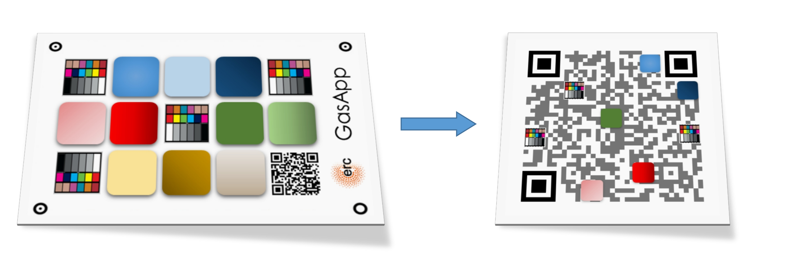
To solve those challenges, we proposed the creation of an integrated machine-readable pattern based on QR Codes, which would embed both the color correction patches and the colorimetric indicators patches. And, those embeddings ought to be back-compatible with the QR Code standard, to maintain the data storage capabilities of QR Codes for traceability applications [20]. A representation of this idea is portrayed in [fig:thesis_proposal].
The novelty of the idea led us to submit a patent application in 2018, which was granted worldwide in 2019, and now is being evaluated in National phases [23]. Moreover, we launched ColorSensing, a spin-off company from Universitat de Barcelona to develop further the technology in industrial applications [24].
The strong points of the back-compatible proposal were:
the use of pre-existent computer vision algorithms to locate QR Codes, freeing the designed pattern of redundant computer vision features, as those ’circles’ seen outside the GasApp card ([fig:thesis_proposal]), which are redundant with the finder patterns of the QR Code (corners of the QR Code);
the reduced size presented by a QR Code ([fig:thesis_proposal]), the original GasApp proposal was set to a business card size (\(\mathrm{3.5}\) \(\times\) \(\mathrm{2.0}\) inches), while our QR Code proposal is smaller (\(\mathrm{1}\) \(\times\) \(\mathrm{1}\) inch);
reducing the barrier between the new technology and the final users, as the back-compatible proposal maintains the mainstream standard of the QR Codes. By this, one could simply encode a desired URL in the QR Code data alongside with the color information and always be able to redirect the final user to a download link of the proper reader, which enables the color readout;
and, the capacity to increase the color references embedded in a color chart, while also reducing the global size of the chart, (e.g. the usual size of a commercial ColorChecker is about 11 \(\times\) 8.5 inches, and it encodes 24 color patches), using modern machine-readable standard (such as QR Codes as an encoding base) enables a systematic path to increase the capacity per surface unit, and subsequently according to color correction theory, leading to a better color corrections having more color references.
All in all, this thesis proposes a new approach to automate color correction for colorimetry applications using barcodes; namely, Color QR Codes featuring colorimetric indicators. Let us enumerate the objectives of the thesis:
To capture machine-readable patterns placed on top of challenging surfaces, which are captured with handheld smartphones. These surfaces can be non-rigid surfaces present in real-world applications, such as: bottles, packaging, food, etc.
To define a back-compatible QR Code modification method to extend QR Codes to act as color charts, which back-compatibility ensures that the digital data of the QR Code remains readable during the whole modification process.
To achieve image consistency using color charts for any camera or light setup, enabling colorimetric applications to yield quantitative results, and doing so by specifying a color correction method that takes into account arbitrary modifications in the captured scene, such as: light source, smartphone device, etc.
To demonstrate a specific application of the technology based on colorimetric indicators, where the accumulated results from objectives I to III are applied.
In this thesis, we tackled the above-mentioned objectives. Prior to that, we introduce in a dedicated chapter the backgrounds and methods applied to this thesis. Then, we present four thematic chapters related to each one of the objectives. These chapters were prepared with a coherent structure: a brief introduction, a proposal, an experimental details section, the results presentation and the conclusion discussion. Later, a general conclusion chapter was added to close the thesis. Let us briefly present the content of each thematic chapter.
First, in [ch:4] we reviewed the state-of-the-art method to extract QR Codes from different surfaces. Then, we focused on a novel approach to readout QR Codes on challenging surfaces, such as those found in food packages, cylinders or any non-rigid plastic [25], [26].
Second, in [ch:5] we introduced the main proposal of the thesis, the back-compatible Color QR Codes [23]. Here, we also introduced not only the machine-readable pattern proposal but also we benchmarked the different possible approaches to embed colors in a QR Code by taking into account its data encoding (i.e. which colors are to be embedded where, etc.) and how it affected the QR Code final readability.
Third, in [ch:6] we sought for a unified framework of color correction based on affine [14], polynomial [27], [28], root-polynomial [28] and thin-plate splines [15] color corrections. Within that framework, we presented our new proposal for an improved TPS3D method to achieve image consistency.
Finally, in [ch:7] we surveyed the different color sensors where we already used partial approaches to our solution [29], [30]. Then, we studied how tho apply our proposal to an actual application of a colorimetric indicator that sensed \(CO_2\) concentrations [31] in modified atmosphere packaging (MAP) [32].
Color reproduction is one of the most studied problems in the audiovisual industry, that is present in our daily lives, long before today’s smartphones, when color was introduced to the cinema, color analog cameras and color home TVs [11]. In the past years, reproducing and measuring color has also become an important challenge for other industries such as health care, food manufacturing and environmental sensing. Regarding health care, dermatology is one of the main fields where color measurement is a strategic problem, from measuring skin-tones to avoid dataset bias [33] to medical image analysis to retrieve skin lesions [34], [35]. In food manufacturing, color is used as an indicator to solve quality control and freshness problems [36]–[38]. As for environmental sensing [4], colorimetric indicators are widely spread to act as humidity [39], temperature [40] and gas sensors [41], [42].
In this section, we focus on image consistency, a reduced problem from color reproduction. While color reproduction aims at matching the color of a given object when reproduced in another device as an image (e.g. a painting, a printed photo, a digital photo on a screen, etc.), image consistency is the problem of taking different images of the same object in different illumination conditions and with different capturing devices, to finally obtain the same apparent colors for that object. In this problem, the apparent colors of an object do not need to match its “real” spectral color, they rather have to be just similar in each instance captured in different scenarios. In other words, all instances should match the first capture, or the reference capture, and not the real-life color. Therefore, image consistency is the actual problem to solve in the before-mentioned applications, in which it is more important to compare acquired images between them, so that consistent conclusions can be drawn with all instances, than comparing them to an actual reflectance spectrum.
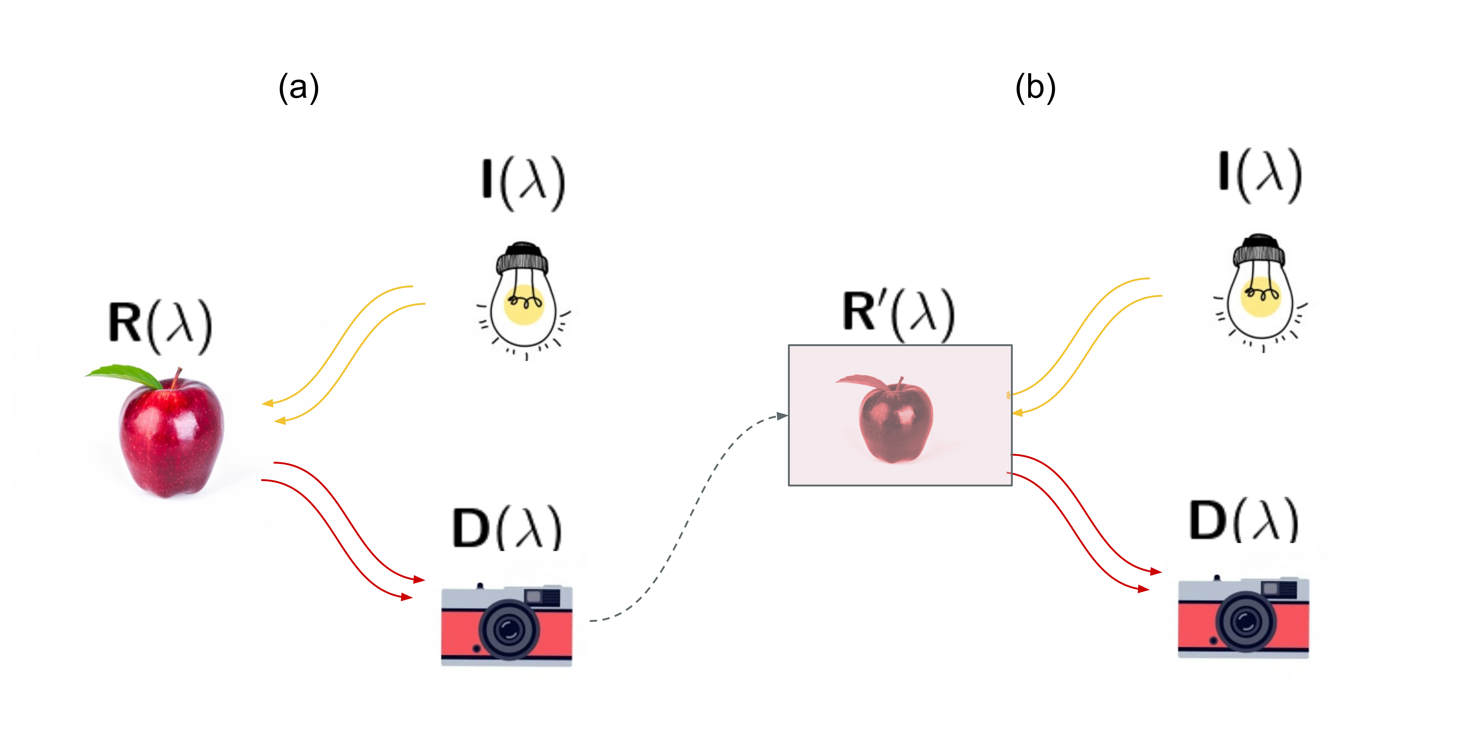
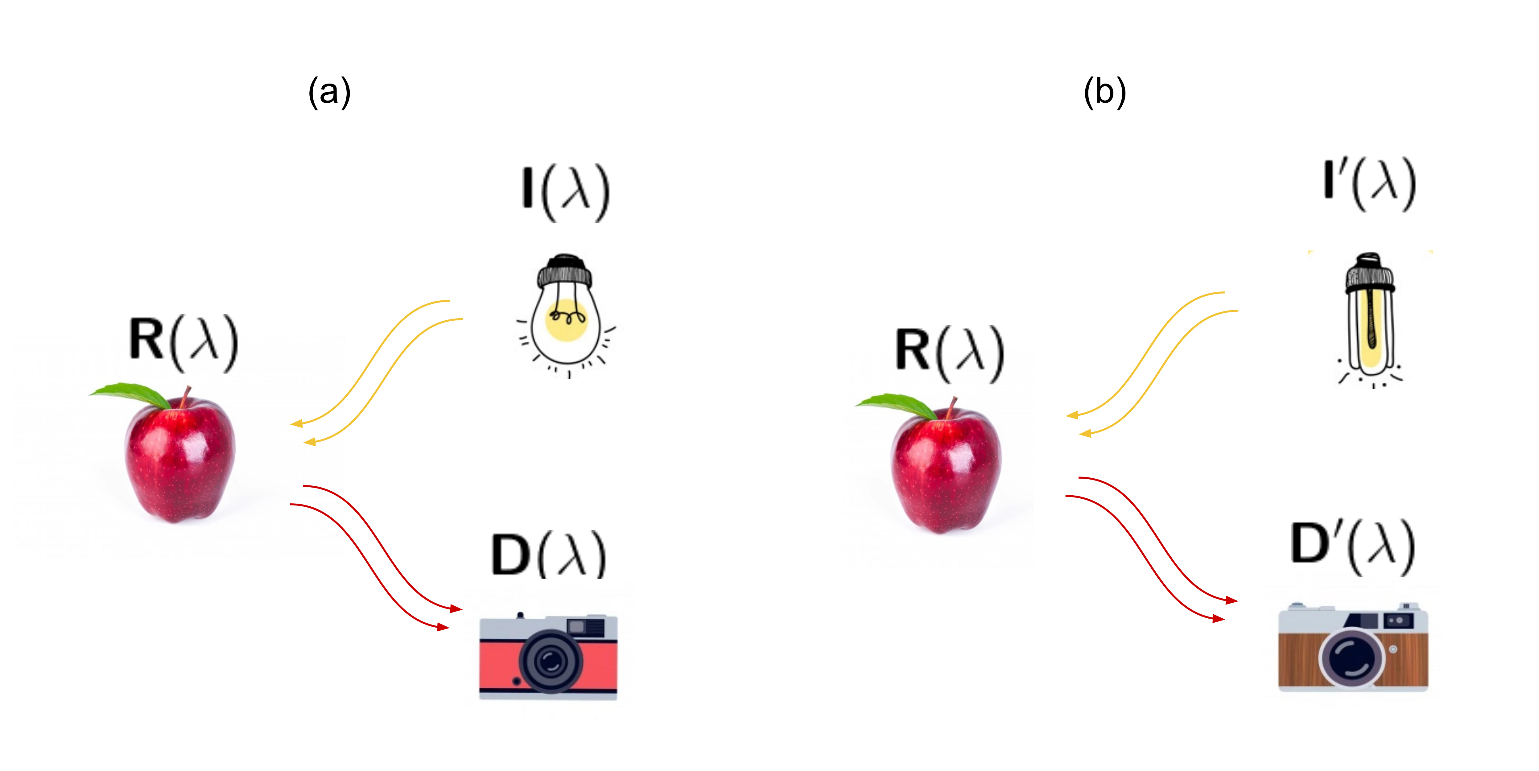
Color reproduction is the problem of matching the reflectance of an object with an image of this object [11]. This can be seen in [fig:colorreproduction].a, where an object (an apple), with a reflectance \(\mathrm{R (\uplambda)}\), is illuminated by a light source \(\mathrm{I (\uplambda)}\) and captured by a camera with a sensor response \(\mathrm{D (\uplambda)}\). In fact, digital cameras contain more than one sensor targeting different ranges of the visible spectrum: commonly, 3 types of sensors centered in red, green and blue colors [11].
In general, the signal acquired by one of the sensors inside the camera device can be modeled as [43]:
\[\mathrm {S_k \propto \int_{-\infty}^{\infty} I(\uplambda) \ R(\uplambda) \ D_k(\uplambda) \ d\uplambda} \label{eq:colorsingalintegral}\]
where \(k \in \{ 1, \dots , \ N \}\) are the channels of the camera, \(N\) is the total number of channels and \(\mathrm{\uplambda}\) are the visible spectra wavelengths. Then, [fig:colorreproduction].b portrays the color reproduction of the object, where now a new reflectance will be recreated and captured with the same conditions. Since our image is a printed image, the new reflectance will be:
\[\mathrm{R'(\uplambda)} = \sum_{i=0}^{M} f_i (S_1, \dots, S_N) \cdot \mathrm{R_i(\uplambda)} \label{eq:reproductionsum}\]
where \(\mathrm{R_i (\uplambda)}\) are the reflectance spectra of the \(M\) reproduction inks, which will be printed as a function of the acquired \(\mathrm{(S_1, \dots, S_N)}\) channel contributions. The color reproduction problem now can be written as the minimization problem to the distance of both reflectances:
\[\mathrm{\left \| R'(\uplambda) -R(\uplambda) \right \| \rightarrow 0} \label{eq:reproductionmin}\]
for each wavelength, for each illumination and for each sensor. The same formulation could be written when displaying images on a screen by changing \(\mathrm{R (\uplambda)}\) for \(\mathrm{I (\uplambda)}\) of the light emitting screen.
Color reproduction is a wide open problem, and with each step towards its general solution, the goal of achieving image consistency when acquiring image datasets is nearer. Since color reproduction solutions aim at attaining better acquisition devices and better reproduction systems, the need for solving the image consistency problem will eventually disappear. But this is not yet the case.
However, the image consistency problem is far simpler than the color reproduction problem. The image consistency problem can be seen as the problem to match the acquired signal of any camera, under any illumination for a certain object. This can be seen in [fig:imageconsistency].a: an object (an apple), which has a reflectance \(\mathrm{R (\uplambda)}\), is illuminated by a light source \(\mathrm{I (\uplambda)}\) and it is captured by a camera with a sensor response \(\mathrm{D (\uplambda)}\). Now, in [fig:imageconsistency].b, the object is not reproduced but exposed again to different illumination conditions \(\mathrm{I' (\uplambda)}\) and captured by a different camera \(\mathrm{D' (\uplambda)}\).
Under their respective illumination, each camera will follow [eq:colorsingalintegral], providing three different \(\mathrm{S_k}\) channels. Considering we can write a vector signal from the camera as:
\[\mathbf{s} = \mathrm{(S_1, \dots, S_N)} \ \mathrm{,} \label{eq:colorvector}\]
the image consistency problem can be written as the minimization problem to the distance between acquired signals:
\[\left \| \mathbf{s}' - \mathbf{s} \right \| \rightarrow 0 \label{eq:consistencymin}\]
for each camera, for each illumination for a given object.
The image consistency problem is easier to solve, as we have changed the problem from working with continuous spectral distributions (see [eq:reproductionmin]) to N-dimensional vector spaces (see [eq:consistencymin]). These spaces are usually called color spaces, and the mappings between those spaces are usually called color conversions. Deformations or corrections inside a given color space are often referred to as color corrections. In this thesis, we will be using RGB images from digital cameras. Thus, we will work with device-dependent color spaces.
This means that the mappings will be performed between RGB spaces. Then, we can rewrite the color vector definition for RGB colors following [eq:colorvector] as:
\[\mathbf{s} = \mathrm{(r, g, b),} \ \ \mathbf{s} \in \mathbb{R}^3 \ \mathrm{,} \label{eq:colorvectorrgb}\]
where \(\mathbb{R}^3\) represents here a generic 3-dimensional RGB space. In [subsec:colorspaces], we detail how color spaces are defined according to their bit resolution and color channels.
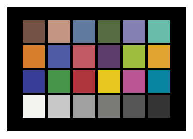
The traditional approach to achieve a general purpose color correction is the use of color rendition charts, introduced by C.S. McCamy et. al. in 1976 [13] (see [fig:colochecker]). Color charts are machine-readable patterns placed in a scene that embed reference patches of a known color, where in order to solve the problem, several color references are placed in a scene to be captured and then used in a post-capture color correction process.
These color correction processes involve algorithms to map the color references seen in the chart to their predefined nominal colors. This local color mapping is then extrapolated and applied to the whole image. There exists many ways to correct the color of images to achieve consistency.
The most extended way to do so is to search for device-independent color spaces (i.e. CIE Lab, CIE XYZ, etc.) [11]. But in the past decade, there have appeared solutions that involve direct corrections between device-dependent color spaces, without the need to pass through device-independent ones.
The most simple color correction technique is the white balance, that only involves one color reference [44]. A white reference inside the image is to be mapped to a desired white color and then the entire image is transformed using a scalar transformation. Beyond that, other techniques that use more than one color reference can be found elsewhere, using affine [44], polynomial [27], [28], root-polynomial [28] or thin-plate splines [15] transforms.
It is safe to say that, in most of these post-capture color correction techniques, increasing the number and quality of the color references offers a systematic path towards better color calibration results. This strategy however, comes along with more image area dedicated to accommodate these additional color references and therefore, a compromise must be found.
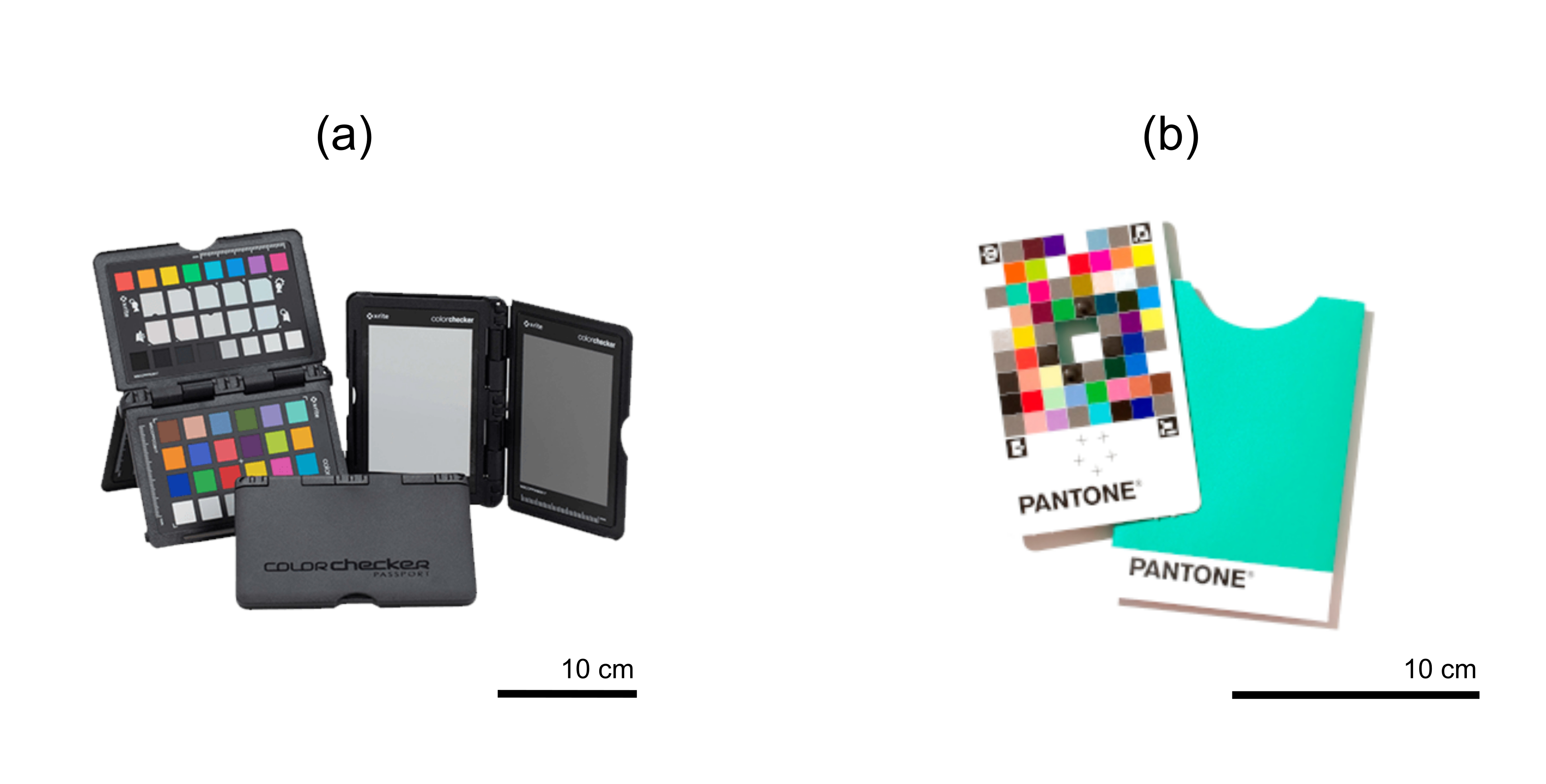
This led X-Rite (a Pantone subsidiary company), to introduce improved versions of the ColorChecker, like the ColorChecker Passport Photo 2 ® kit (see Figure 4.a). Also in this direction, Pantone presented in 2020 an improved color chart called Pantone Color Match Card ® (see Figure 4.b), based on the ArUco codes introduced by S. Garrido-Jurado et al. in 2015 [19] to facilitate the location of a relatively large number of colors. Still, the size of these color charts is too big for certain applications with size constraints (e.g. smart tags for packaging [30], [45]).
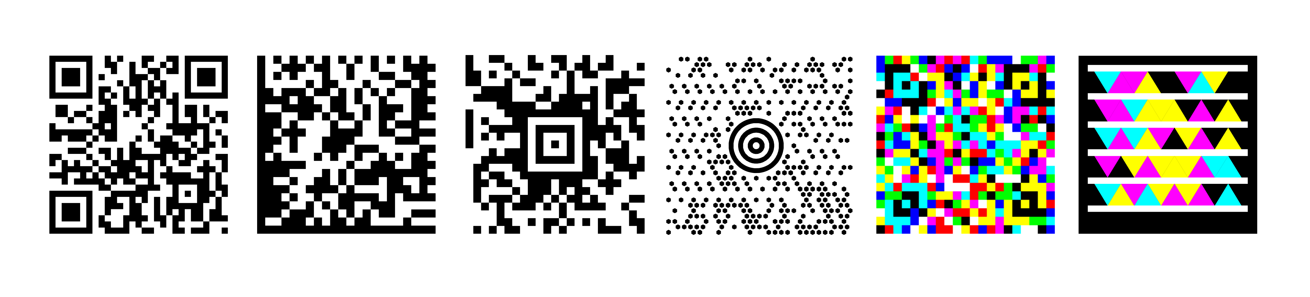
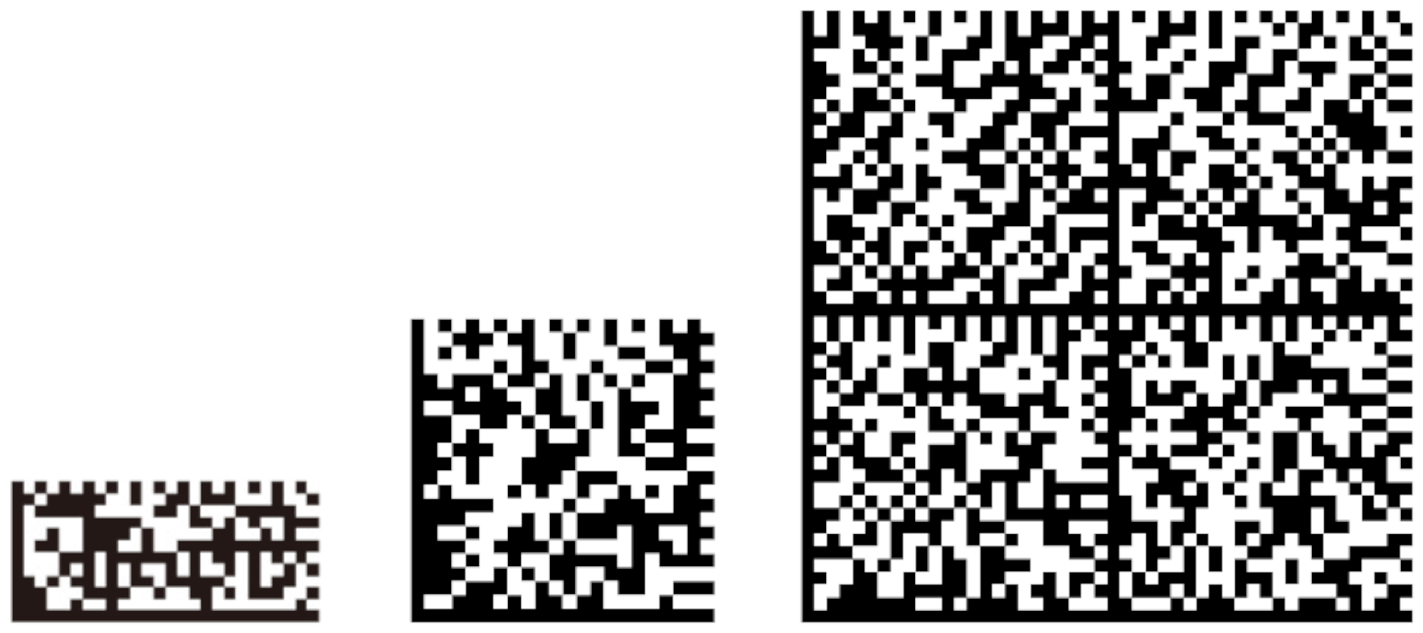
Quick-Response Codes, popularized as QR Codes, are 2D barcodes introduced in 1994 by Denso Wave [20], which aimed at replacing traditional 1D barcodes in the logistic processes of this company. However, the use of QR Codes has escalated in many ways and are now present in manifold industries: from manufacturing to marketing and publicity, becoming a part of the mainstream culture. In all these applications, QR Codes are either printed or displayed and later acquired by a reading device, which normally includes a digital camera or barcode scanner. Also, there has been an explosion of 2D barcode standards [46]–[50] (see [fig:2dbarcodes]).
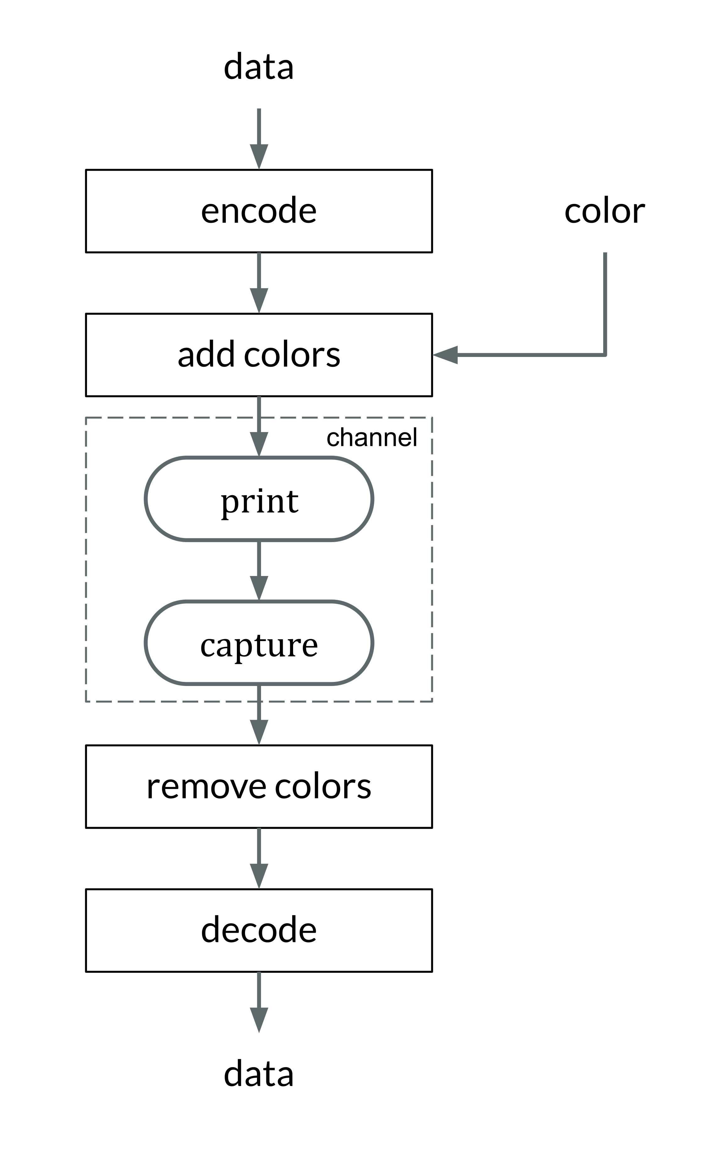
The process of encoding and decoding a QR Code could be considered as a form of communication through a visual channel (see [fig:defaultqrflow]): a certain message is created, then split into message blocks, these blocks are encoded in a binary format, and finally encoded in a 2D array. This 2D binary array is an image that is transmitted through a visual channel (printed, observed under different illuminations and environments, acquired as a digital image, located, resampled, etc.). On the decoder side, the binary data of the 2D binary array is retrieved, the binary stream is decoded, and finally the original message is obtained.
From the standpoint of a visual communication channel, many authors before explored the data transmission capabilities of the QR Codes, especially as steganographic message carriers (data is encoded in a QR Code, then encoded in an image) due to their robust error correction algorithm [51], [52].
Many 2D barcode standards allow modulating the amount of data encoded in the barcode. For example, the QR Code standard implements different barcode versions from version 1 to version 40. Each version increases the edges of the QR Code by 4 pixels, the so-called modules. From the starting \(\mathrm{21 \times 21}\) (\(\mathrm{v1}\)) modules up to \(\mathrm{144 \times 144}\) modules (\(\mathrm{v40}\)) [20].
For each version, the location of every computer vision feature is fully specified in the standard (see [fig:qrversions]), in [subsec:qrfeatures] we will focus on these features. Some other 2D barcode standards are flexible enough to cope with different shapes, such as rectangles in the DataMatrix codes (see [fig:dmversions]), which can be easier to adapt to different substrates or physical objects [46].

These different possible geometries must be considered when adding colors to a 2D barcode. In the case of the QR Codes and DataMatrix codes, the larger versions are built by replicating a basic squared block. Therefore, the set of color references could be replicated in each one of these blocks, to gain in redundancy and in a more local color correction. Alternatively, different sets of color references could be used in each periodic block to facilitate a more thorough color correction based on a larger set of color references.
Regarding this size and shape modularity in 2D barcode encoding, there exist a critical relationship between the physical size of the modules and the pixels in a captured image. This is a classic sampling phenomena [53]: for a fixed physical barcode size and a fixed capture (same pixels), as the version of the QR Code increases the amount of modules in a given space increases as well.
Thus, when the apparent size of the module in the captured image decreases, the QR Code module is hardly a bunch of image pixels, and we start to see aliasing problems [54]. In turn, this problem leads to a point where QR Codes cannot be fully recognized by the QR Code decoding algorithm. This is even more important if we substitute these black and white modules with colors, where the error in finding the right reference area may lead to huge errors in the color evaluation. Therefore, this sampling problem will accompany the implementation of our proposal taking into account the size of the final QR Code depending on the application field and the typical resolution of the cameras used in those applications.
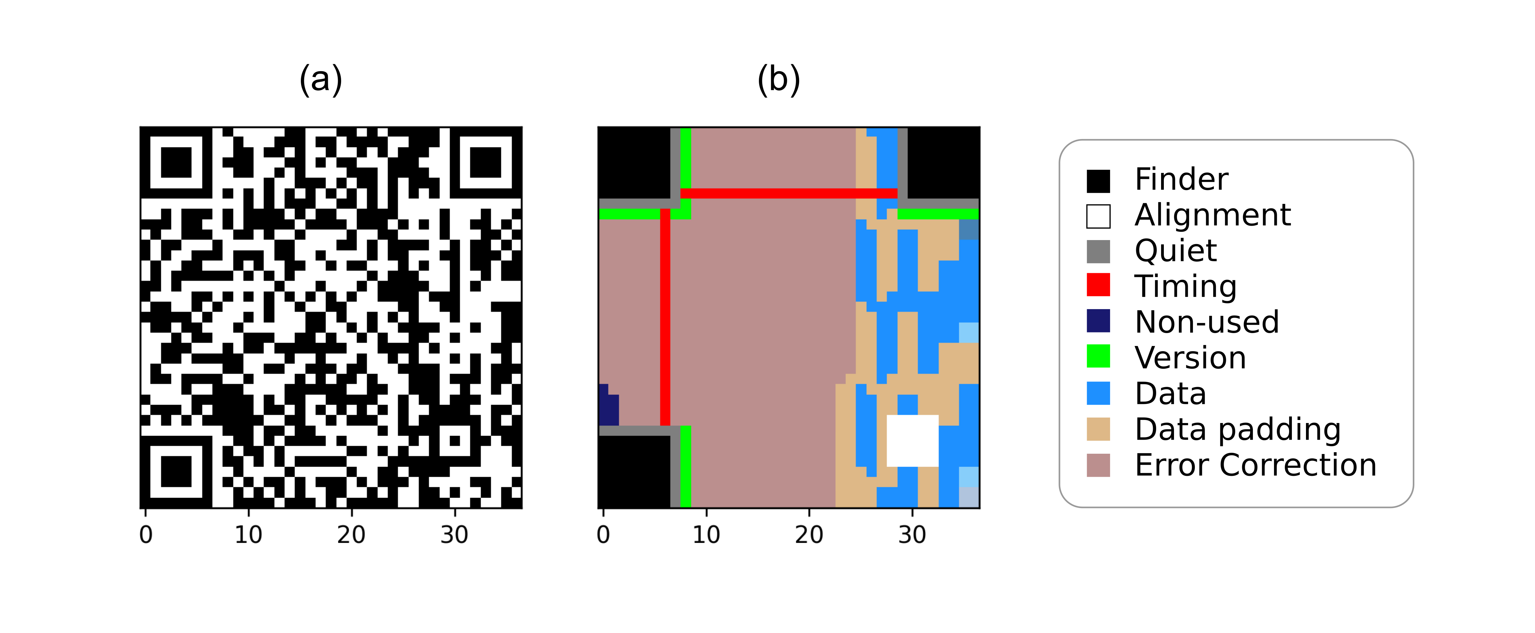
The QR Code standard presents a complex encoding layout (see [fig:qrencoding]). Encoding a message into a QR Code form implies several steps.
First, the message is encoded as binary data and split into various bytes, namely data blocks. Since QR Codes can support different data types, the binary encoding for those data types will be different in order to maximize the amount of data to encode in the barcode (see [tab:qrcapacity]).
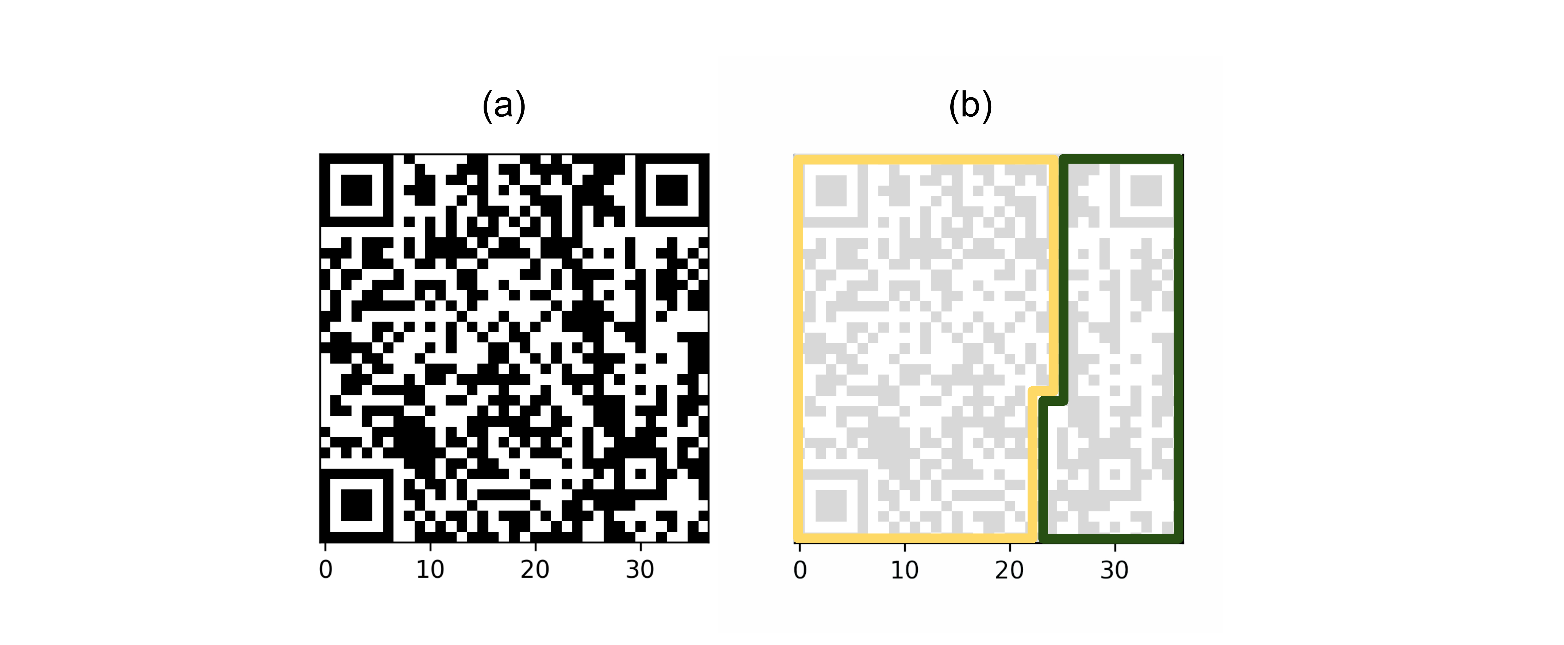
Second, additional error correction blocks are computed based on the Reed-Solomon error correction theory [55]. Third, the minimal version of the QR Code is determined, which defines the size of the 2D array to “print” the error correction and data blocks, as a binary image. When this is done, the space reserved for the error correction blocks is larger than the space reserved for the data blocks (see [fig:qrencodingsimple]).
Finally, a binary mask is implemented in order to randomize as much as possible the QR Code encoding [20].
During the generation of a QR Code, the level of error correction (ECC) can be selected, from high to low capabilities: H (30 %), Q (25%), M (15%) and L (7%). This should be understood as the maximum number of error bits that a certain barcode can support (maximum Bit Error Ratio, detailed in [ch:5]). Notice the error correction capability is independent of the version of the QR Code. However, both combined define the maximum data storage capacity of the QR Code. For a fixed version, higher error correction implies a reduction of the data storage capacity of the QR Code.
This error correction feature is indirectly responsible for the popularity of QR Codes, since it makes them extremely robust while allowing for a large amount of pixel tampering to accommodate aesthetic features, like allocating brand logos inside the barcode [56], [57] (see [fig:qrswithlogos] and [fig:qrswithlogoscolor]). In this thesis, we will take advantage of such error correction to embed reference colors inside a QR Code.
![Different examples of Halftone QR Codes, introduced by HK. Chu et al. [56]. These QR Codes exploit the error correction features of the QR Code to achieve back-compatible QR Codes with apparent grayscale –halftone– colors.](assets/graphics/chapters/chapter3/figures/jpg/halftone_qrcodes.jpg)
![Original figure from Garateguy et al. (© 2014 IEEE) [57], different QR Codes with color art are shown: (a) a QR Code with a logo overlaid; (b) a QArt Code [58], (c) a Visual QR Code; and (d) the Garateguy et al. proposal.](assets/graphics/chapters/chapter3/figures/jpg/garateguy.jpg)
Besides the data encoding introduced before, a QR Code embeds computer vision features alongside with the encoded digital data. These features play a key role when applying computer vision transformations to the acquired images containing QR codes. Usually, they are extracted to establish a correspondence between their apparent positions in the captured image plane and those in the underlying 3D surface topography. The main features we focus on this thesis are:
Finder patterns are the corners of the QR Code, it has 3 of them to break symmetry and orient the QR in a scene (see [fig:qrcodeparts].a).
Alignment patterns are placed inside the QR Code to help in the correction of noncoplanar deformations (see [fig:qrcodeparts].b).
Timing patterns are located alongside two borders of the QR Code, between a pair of finder patterns, to help in the correction of coplanar deformations (see [fig:qrcodeparts].c).
The fourth corner is the one corner not marked with a finder pattern. It can be found as the crosspoint of the straight extensions of the outermost edges of two finder patterns (see [fig:qrcodeparts].d). It is useful in linear, coplanar and noncoplanar deformations.
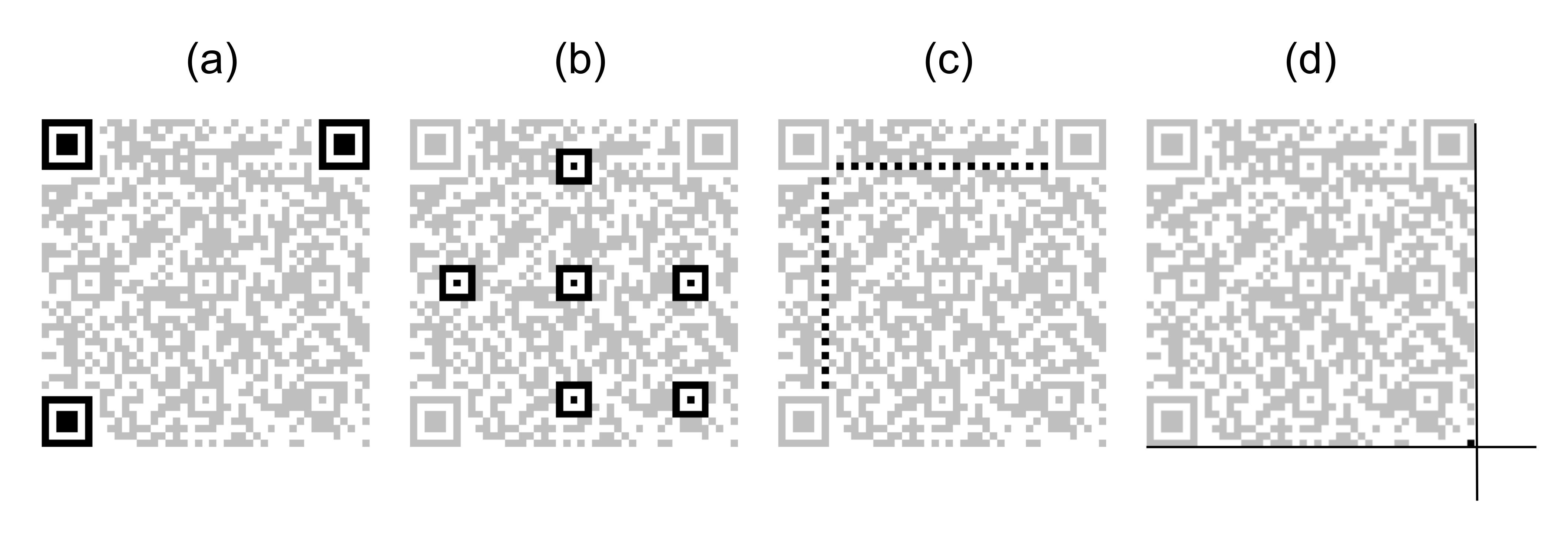
These features are easy to extract due to their spatial properties. They are well-defined as they do not depend on the version of the QR Code, nor the data encoding. The lateral size for a finder pattern is always \(\mathrm{7}\) modules. For an alignment pattern, \(\mathrm{5}\) modules. And timing patterns grow along with each version, but their period is always \(\mathrm{2}\) modules (one black, one white).
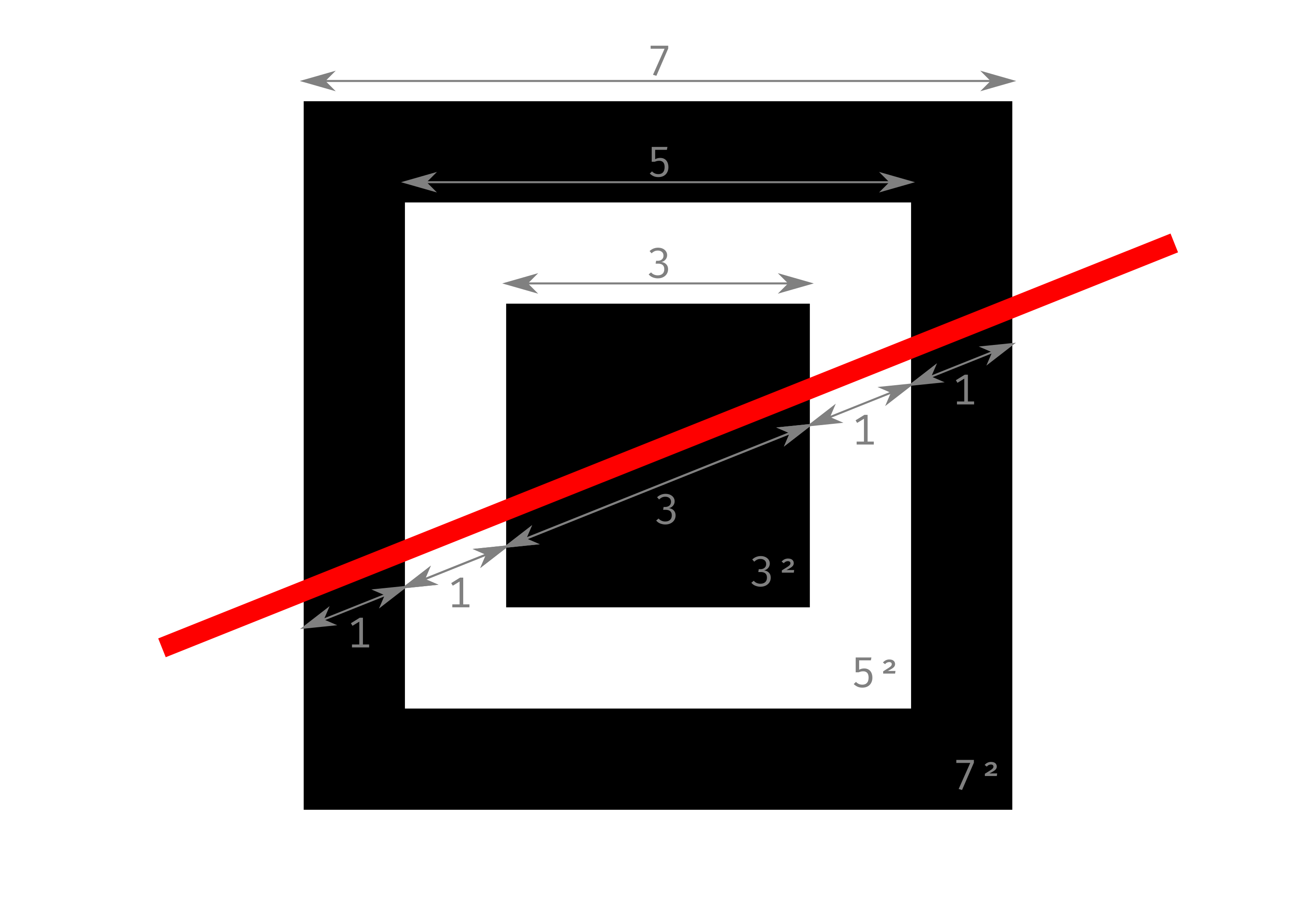
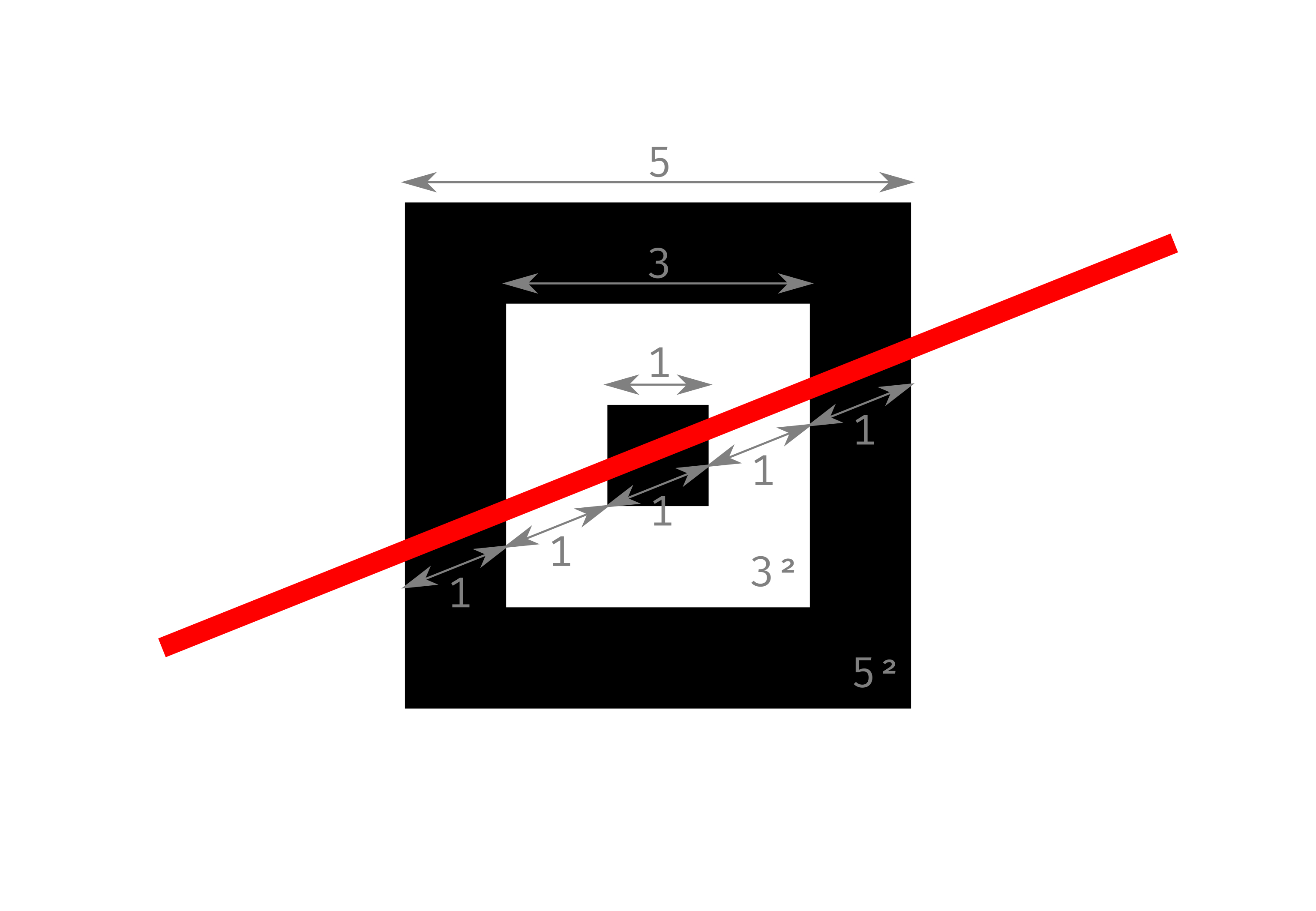
Finder patterns implement a sequence of modules along both axes that follows: \(\mathrm{1}\) black, \(\mathrm{1}\) white, \(\mathrm{3}\) black, \(\mathrm{1}\) white and \(\mathrm{1}\) black, often written as a \(\mathrm{1:1:3:1:1}\) relation (see [fig:finderpattern]). Alignment patterns implement a sequence of modules along both axes that follows: \(\mathrm{1}\) black, \(\mathrm{1}\) white, \(\mathrm{1}\) black, \(\mathrm{1}\) white and \(\mathrm{1}\) black, a \(\mathrm{1:1:1:1:1}\) relation (see [fig:alignmentpattern]).
Thus, the relationship between white and black pixels provides a path to use pattern recognition techniques to extract these features, as these relations are invariant to perspective transformations. Moreover, these linear relations can be expressed as squared area relations, and are still invariant under perspective transformations. This is specially useful when using extraction algorithms based upon contour recognition [18], [59]. For finder patterns the area relation becomes \(\mathrm{7^2:5^2:3^2}\) (see [fig:finderpattern]); and for alignment patterns, \(\mathrm{5^2:3^2:1^2}\) (see [fig:alignmentpattern]).
Let us explore a common pipeline towards QR Code readout. First, consider a QR Code captured from a certain point-of-view in a flat surface which is almost coplanar to the capture device (e.g. a box in a production line). Note that more complex applications, such as bottles [60], all sorts of food packaging [61], etc., which are key to this thesis, are tackled in [ch:4].
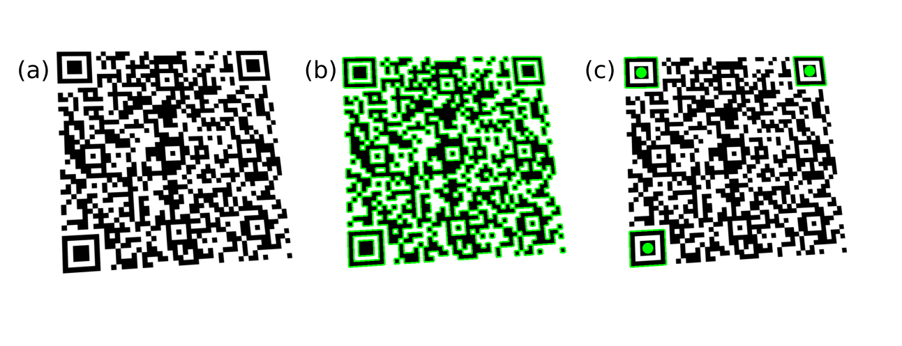
Due to perspective, the squared shape of the QR Code will be somehow deformed following some sort of projective transformation (see [fig:qrcontours].a). Then, in order to find the QR Code itself within the image field, the three finder patterns are extracted applying contour recognition algorithms based on edge detection [18], [59] (see [fig:qrcontours].b). As explained in [subsec:qrfeatures], each finder pattern candidate must hold a very specific set of area relationships, no matter how they are projected if the projection is linear. The contours that fulfill this area relationship are labeled as candidates finder patterns (see [fig:qrcontours].c).
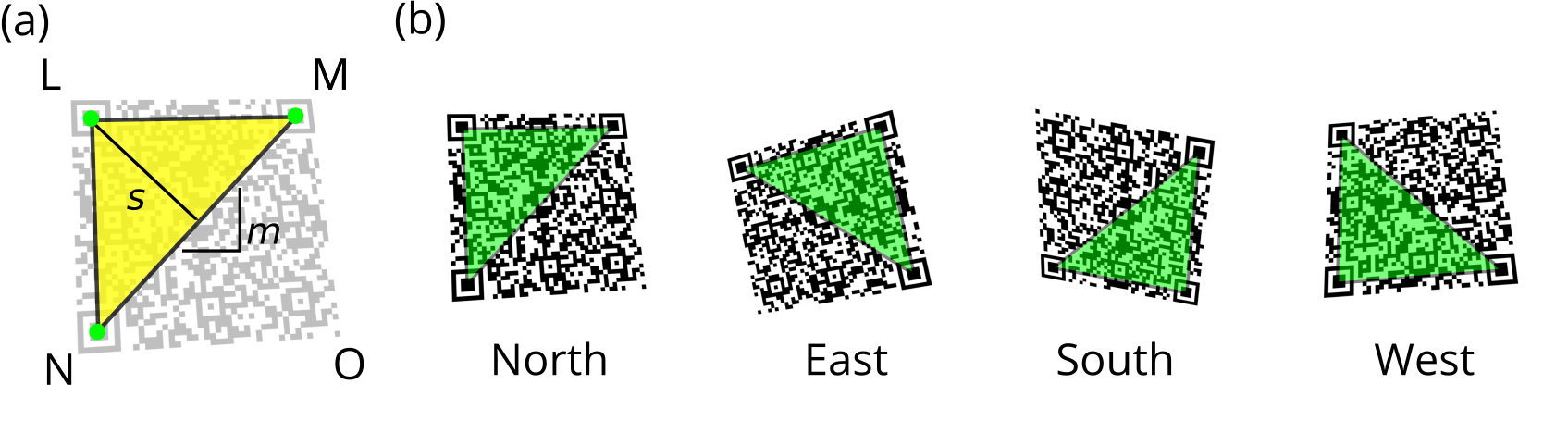
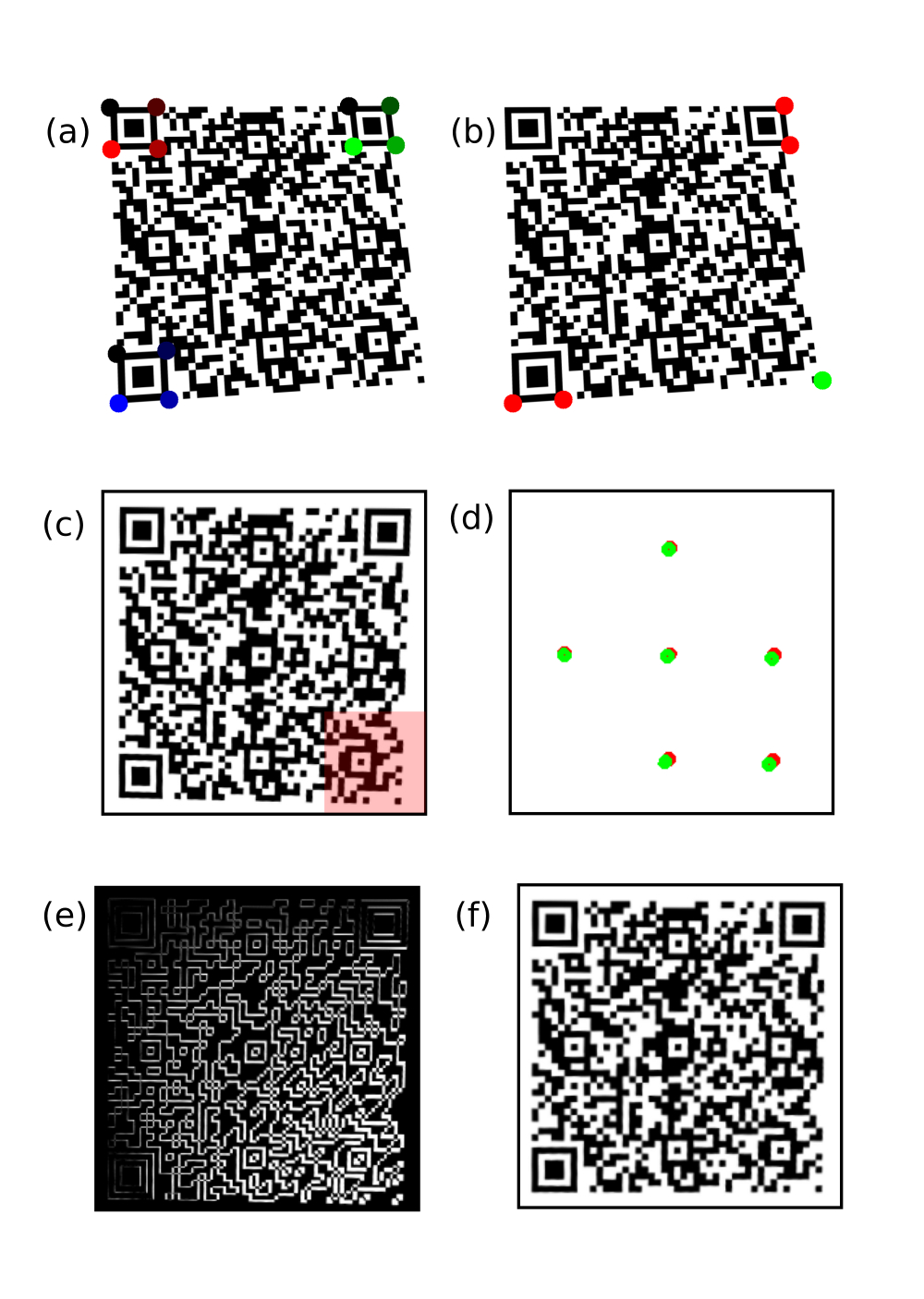
Second, the orientation of the QR Code must be recognized, as in a general situation, the QR Code captured in an image can take any orientation (i.e. rotation). The above-mentioned three candidate finder patterns are used to figure out the orientation of the barcode. To do so, we should bear in mind that one of these corners will correspond to the top-left one and the other two will be the end points of the opposite diagonal (see [fig:qrorientation].a). By computing the distances between the three candidate finder pattern centers and comparing them we can find which distance corresponds to the diagonal and assign the role of each pattern in the QR Code accordingly. The sign of the slope of the diagonal \(m\) and the sign of the distance to the third point \(s\) are computed and analyzed to solve the final assignment of the patterns. The four possible combinations result in 4 possible different orientations: north, east, south, west (see [fig:qrorientation].b). Once the orientation is found, the three corner candidates are labeled following the sequence \({L, M, N}\).
Third, a projection correction is performed to retrieve the QR Code from the scene. The finder patterns can then be used to correct the projection deformation of the image in the QR Code region. If the deformation is purely affine, e.g. a flat surface laying coplanar to the reader device, we can perform the correction with these three points. But, if a more general deformation is presented, e.g. handheld capture in a perspective plane, one needs at least one additional point to carry out such transformation: the remaining fourth corner \(O\) (see [fig:qrorientation].a). As the edges around the 3 main corners were previously determined (see [fig:qrcorrectperspective].a), the fourth corner \(O\) is localized using the crossing points of two straight lines from corners \(M\) and \(N\) (see [fig:qrcorrectperspective].b). With this set of 4 points, a projective transformation that corrects the perspective effect on the QR Code can also be carried out (see [fig:qrcorrectperspective].c).
Notice the calculation of the fourth corner \(O\) can accumulate the numerical error of the previous steps. This might lead to inaccurate results in the bottom-right corner of the recovered code (see [fig:qrcorrectperspective].c) and, in some cases, to a poor perspective correction. This effect is especially strong in low resolution captures, where the modules of the QR Code measure a few image pixels. In order to solve this issue, the alignment patterns are localized (see [fig:qrcorrectperspective].d) in a more restricted and accurate contour search around the bottom-right quarter of the QR Code (see [fig:qrcorrectperspective].e). With this better estimation of a grid of reference points of known (i.e. tabulated) positions a second projective transformation is carried out (see [fig:qrcorrectperspective].f). Normally, having more reference points than strictly needed to compute projective transformations is not a problem thanks to the use of maximum likelihood estimation (MLE) solvers for the projection fitting [62].
Finally, the QR Code readout is performed, this means the QR Code is down-sampled to a resolution where each of the modules occupies exactly one image pixel. After this, the data is extracted following a reverse process of the encoding: the data blocks are interpreted as binary data, also the error correction blocks. The Reed-Solomon technique to resolve errors is applied, and the original data is retrieved.
In [sec:theimageconsistency] we introduced the image consistency problem alongside with a simplified description of the reflectance model (see [fig:colorreproduction_mini]):
\[\mathrm {S_k \propto \int_{-\infty}^{\infty} I(\uplambda) \ R(\uplambda) \ D_k(\uplambda) \ d\uplambda} \label{eq:colorsingalintegral_bis}\]
where a certain light source \(\mathrm{I} (\uplambda)\) illuminates a certain object with a certain reflectance \(\mathrm{R} (\uplambda)\) this scene is captured by a sensor with its response \(\mathrm{D_k} (\uplambda)\); and \(\mathrm {S_k}\) represents the signal captured by this sensor. This model specifically links the definition of color to the sensor response, not only to the wavelength distribution of the reflected light. Thus, our color definition depends on the observer.
Let the sensor \(\mathrm{D_k} (\uplambda)\) be the human eye, then this model becomes the well-known tristimulus model of the human eye. In the tristimulus model, a standard observer is defined from studying the human vision. In 1931 the International Commission of Illumination defined the CIE 1931 RGB and CIE 1931 XYZ color spaces based on the human vision [63], [64]. Since then, the model has been revisited many times defining new color spaces: in 1960 [65], in 1964 [66], in 1976 [67] and so on [68].
Commonly, color spaces referred to a standard observer are called device-independent color spaces. As explained before, we are going to use images which are captured by digital cameras. These images will use device-dependent color spaces, despite the efforts of their manufacturers to solve the color reproduction problem, as they try to match the camera sensor to the tristimulus model of the human eye [69].
Let a color \(\mathbf{s}\) be defined by the components of the camera sensor:
\[\mathbf{s} = (\mathrm{S_r}, \ \mathrm{S_g}, \ \mathrm{S_b}) \label{eq:scolor}\]
where \(\mathrm{S_r}\) , \(\mathrm{S_g}\) and \(\mathrm{S_b}\) are the responses of the three sensors of the camera for the red, green and blue channels, respectively. Cameras do imitate the human tristimulus vision system by placing sensors in the wavelength bands representing those where human eyes have more sensitivity.
Note that \(\mathbf{s}\) is defined as a vector in [eq:scolor]. Although, its definition lacks the specification of its vector space:
\[\mathbf{s} = (r, \ g, \ b) \ \in \mathbb{R}^3 \label{eq:scolor_vector}\]
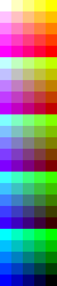
where \(r\), \(g\), \(b\) is a simplified notation of the channels of the color, and \(\mathbb{R}^3\) is a generic RGB color space. As digital cameras store digital information in a finite discrete representation, \(\mathbb{R}^3\) should become \(\mathbb{N}^3_{[0, 255]}\) for 8-bit images (see [fig:rgb_cube]). This discretization process of the measured signal in the camera sensor is a well-known phenomenon in signal-processing, it is called quantization [70]. All to all, we can write some common color spaces in this notation:
\(\mathbb{N}_{[0, 255]}\) is the grayscale color space of 8-bit images.
\(\mathbb{N}^3_{[0, 255]}\) is the RGB color space of 24-bit images (8-bits/channel).
\(\mathbb{N}^3_{[0, 4096]}\) is the RGB color space of 36-bit images (12-bits/channel).
\(\mathbb{N}^3_{[0, 65536]}\) is the RGB color space of 48-bit images (16-bits/channel).
\(\mathbb{N}^4_{[0, 255]}\) is the CMYK color space of 32-bit images (8-bits /channel).
\(\mathbb{R}^3_{[0, 1]}\) is the RGB color space of a normalized image, specially useful when using computer vision algorithms.
The introduction of color spaces as vector spaces brings all the mathematical framework of geometric transformations. We can now define a color conversion as the application between two color spaces.
For example, let \(f\) be a color conversion between an RGB and a CMYK space:
\[f: \mathbb{N}^3_{[0, 255]} \to \mathbb{N}^4_{[0, 255]}\]
this color conversion can take any form. In [sec:theimageconsistency], we saw that the reflectance spectra of the image of an object would be a linear combination of the inks reflectance spectra used to reproduce that object. If we recover that expression from [eq:reproductionsum] and combine it with the RGB color space from [eq:scolor_vector], we obtain:
\[\mathrm{R'(\uplambda)} = \sum_{j}^{c,m,y,k} f_j (r, g, b) \cdot \mathrm{R_j(\uplambda)} \label{eq:reproductionsum_bis}\]
Now, \(\mathrm{R'(\uplambda)}\) is a linear combination of the reflectance spectra of the cyan, magenta, yellow and black inks. The weights of the combination is the CMYK color derived from the RGB color.
In turn, we can express the CMYK color also as a linear combination of the RGB color channels, \(f_i (r, g, b)\) is our color correction here, then:
\[\mathrm{R'(\uplambda)} = \sum_{j}^{c,m,y,k} \left[ \sum_{k}^{r,g,b} a_{jk} \cdot k \right] \cdot \mathrm{R_j(\uplambda)} \label{eq:reproductionsum_rgb}\]
Note that we have defined \(f_i\) as a linear transformation between the RGB and the CMYK color spaces. Doing so is the most common way to perform color transformations between color spaces.
These are the foundations of the ICC Profile standard [71]. Profiling is a common technique when reproducing colors. For example, take [fig:rgb_cube], if the colors are seen displayed on a screen they will show the RGB space of the LED technology of the screen. However, if they have been printed, the actual colors the reader will be looking at will be the linear combination of CMYK inks representing the RGB space, following [eq:reproductionsum_rgb]. Therefore, ICC profiling is present in each color printing process.
Alongside with the described example, here below, we present some of the most common color transformations we will use during the development of this thesis, that include normalization, desaturation, binarization and colorization transformations.
Normalization is the process of mapping a discrete color space with limited resolution (\(\mathbb{N}_{[0, 255]}\), \(\mathbb{N}^3_{[0, 255]}\), \(\mathbb{N}^3_{[0, 4096]}\), ...) into a color space which is limited to a certain range of values, normally from 0 to 1 \(\mathbb{R}_{[0, 1]}\), but offers theoretically infinite resolution 1. All our computation will take place in such normalized spaces. Formally the normalization process is a mapping that follows:
\[f_{normalize} : \mathbb{N}^K_{[0, \ 2^n]} \to \mathbb{R}^K_{[0, 1]} \label{eq:color_normalize}\]
where \(K\) is the number of channels of the color space (i.e. \(K = 1\) for grayscale, \(K = 3\) for RGB color spaces, etc.) and \(n\) is the bit resolution of the color space (i.e. 8, 12, 16, etc.).
Note that a normalization mapping might not be that simple so only implies a division by a constant. For example, an image can be normalized using an exponential law to compensate camera acquisition sensitivity, etc. [72], [73].
Desaturation is the process of mapping a color space into a grayscale representation of this color space. Thus, formally this mapping will always be a mapping from a vector field to a scalar field. We will assume the color space has been previously normalized following a mapping (see [eq:color_normalize]). Then:
\[f_{desaturate} : \mathbb{R}^K_{[0, 1]} \to \mathbb{R}_{[0, 1]} \label{eq:color_desaturate}\]
where \(K\) is still the number of channel the input color space has. There exist several ways to desaturate color spaces, for example, each CIE standard incorporates different ways to compute their luminance model [64].
Binarization is the process of mapping a grayscale color space into a binary color space, this means the color space gets reduced only to a representation of two values. Formally:
\[f_{binarize} : \mathbb{R}_{[0, 1]} \to \mathbb{N}_{[0, 1]} \label{eq:color_binarize}\]
Normally, these mappings need to define some kind of threshold to split the color space representation into two subsets. Thresholds can be as simple as a constant threshold or more complex [74].
Colorization is the process of mapping a grayscale color space into a full-featured color space. We can define a colorization as:
\[f_{colorize} : \mathbb{R}_{[0, 1]} \to \mathbb{R}^K_{[0, 1]} \label{eq:color_colorize}\]
where \(K\) is now the number of channels the output color space has. This process is more unusual than the previous mappings presented here. It is often implemented in those algorithms that pursue image restoration [75]. In this work, colorization will be of a special interest in [ch:5].
A digital image is the result of capturing a scene with an array of sensors, e.g. the camera [11], following [eq:colorsingalintegral_bis]. A monochromatic image \(I\), means we only have one color channel in our color space. This image can be seen as a mapping between a vector field, the 2D plane of the array of sensors, and a scalar field, the intensity of light captured by each sensor:

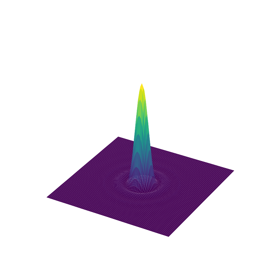
\[I: \mathbb{R}^2 \to \mathbb{R} \label{eq:image_mapping}\]
where \(\mathbb{R}^2\) is the capture plane of the camera sensors and \(\mathbb{R}\) is a generic grayscale color space. [fig:img_vs_profile] shows an example of this: an Airy disk [76] is represented first as an image, where the center of the disk is visualized as a spot; also, the Airy disk is shown to be a function of the space distribution.
Altogether, we can extend [eq:image_mapping] definition to images that are not grayscale. This means each image can be defined as a mapping from the 2D plane of the array of sensors to a color space, which is in turn also a vector space:
\[I: \mathbb{R}^2 \to \mathbb{R}^K\]
where \(\mathbb{R}^K\) is now a vector field also, thus the color space of the image can be RGB, CMYK, etc. Note digital cameras can capture more than the above-mentioned color bands, and there exists a huge field of multi-spectral cameras [77], which is not the focus of our research.
As we pointed out when defining color spaces, digital images are captured using discrete variable color spaces. But this process also affects the spatial domain of the image. The process of discretizing the plane \(\mathbb{R}^2\) is called sampling. And, the process of discretizing the illumination data in \(\mathbb{R}\) data is called quantization. Following this, [eq:image_mapping] can be rewritten as:
\[I: \mathbb{N}_{[0, n]} \times \mathbb{N}_{[0,m]} \to \mathbb{N}_{[0, 255]} \label{eq:image_mapping_discrete}\]
which represents an 8-bit grayscale2 image of size \((n, m)\). This definition of an image allows us to differentiate the domain transformations of the image (i.e. geometrical transformations to the perspective of the image); from the image transformations (i.e. color corrections to the color space to the image).
In [ch:4], when dealing with the extraction of QR Codes from challenging surfaces we used the definition in [eq:image_mapping] to refer to the capturing plane of the image and how it relates to the underneath surface where the QR Code is placed by projective laws.
In [ch:5] we used the definition of [eq:image_mapping_discrete] to detail our proposal for the encoding process of colored QR Codes. In this context, it is interesting reducing the notation of image definition taking into account that images can be regarded as matrices. So, [eq:image_mapping_discrete] can be rewritten in a compact form as:
\[I \in [0, 255]^{n \times m}\]
where \(I\) is now a matrix which exist in a matrix space \([0, 255]^{n \times m}\). This vector space contains both the definition of the spatial coordinates of the image and the color space.
As before, we can use this notation to represent different image examples:
\(I \in [0, 255]^{n \times m}\), is an 8-bit grayscale image with size \((n, m)\).
\(I \in [0, 255]^{n \times m \times 3}\), is an 8-bit RGB image with size \((n, m)\).
\(I \in [0, 1]^{n \times m}\), is a float normalized grayscale image with size \((n, m)\).
\(I \in \{0, 1\}^{n \times m}\), is a binary image with size \((n, m)\).
Finally, we can reintroduce the color space transformations presented before, from [eq:color_normalize] to [eq:color_colorize], for images as bitmap matrices:
Normalization: \[% \label{eq:normalizationdef} f_{normalize}: [0,255]^{n \times m \times 3} \to [0,1]^{n \times m \times 3}\]
Desaturation: \[% \label{eq:desaturationdef} f_{desaturate}: [0,1]^{n \times m \times 3} \to [0,1]^{n \times m}\]
Binarization: \[% \label{eq:binarizationdef} f_{binarize}: [0,1]^{n \times m} \rightarrow \{0,1\}^{n \times m}\]
Colorization: \[% \label{eq:binarizationdef} f_{colorize}: [0,1]^{n \times m} \rightarrow [0,1]^{n \times m \times 3}\]
In 1990, Guido van Rosum released the first version of Python, an open-source, interpreted, high-level, general-purpose, multi-paradigm (procedural, functional, imperative, object-oriented) programming language [78]. Since then, Python has released three major versions of the language: Python 1 (1990), Python 2 (2000) and Python 3 (2008) [79].
At the time we started to work in this thesis, Python was one of the most popular programming languages both in the academia and in the industry [80]. As Python is an interpreted language, the actual code of Python is executed by the Python Virtual Machine (PVM), this opens the door to create different PVM written with different compiled languages, the official Python distribution is based on a C++ PVM, that is why the mainstream Python distribution is called ’CPython’ [81].
CPython allows the user to create bindings to C/C++ libraries, this was specially useful for our research. OpenCV is a widely-known tool-kit for computer vision applications, which is written in C++, but presents bindings to other languages like Java, MATLAB or Python [82].
Altogether, we decided to use Python as our main programming language. Both achieving the rapid script capabilities that Python offers, alongside with standard libraries from Python and C++. The research started with Python 3.6 and ended with Python 3.8, due to the Python’s development cycle.
Let us detail the stack of standard libraries used in the development of this thesis:
Python environment: we started using Anaconda,
an open-source Python distribution that contained pre-compiled packages
ready to be used, such as OpenCV [83]. We adopted also pyenv, a
tool to install Python distributions and manage virtual environments
[84]. Later on, we
started to use docker technology, light virtual machines to
enclose the PVM and our programs [85].
Scientific and data: we adopted the well-known
numpy / scipy / matplotlib
stack:
numpy is a C++ implementation of array
representation (MATLAB-like) for Python [86],
scipy is a compendium of common mathematical
operations fully compatible with NumPy arrays. Often SciPy implements
bindings to consolidated calculus frameworks written in C++ and Fortran,
such as OpenBlas [87],
matplotlib is a 2D graphics environment we used to
represent our data [88].
NumPy, SciPy and Matplotlib are the entry point to a huge ecosystem of packages that use them as their core. When processing datasets, two main packages were used,
pandas is an abstraction layer to the previous
stack, where data is organized in spreadsheets (like Excel, Origin Lab,
etc.) [89],
xarray is another abstraction layer to the previous
stack, with labeled N-dimensional arrays, xarray can be regarded as the
N-dimensional generalization of pandas [90].
Images manipulation: there is a huge ecosystem regarding image manipulation in Python, previous to computer vision, we adopted some packages to read and manipulate images,
pillow is the popular fork from the unmaintained
Python Imaging Library, we used Pillow specially to manipulate the image
color spaces, e.g. profile an image from RGB to be printed in CMYK [91],
imageio was used as an abstraction layer from
Pillow, which uses Pillow and other I/O libraries (such as
rawpy) to read images and convert them directly to NumPy
matrices. We standardized our code to read images using this package
instead of using other solutions (SciPy, Matplotlib, Pillow, OpenCV,
...) [92],
imgaug was used to expand image datasets, by tuning
randomly parameters of the image (illumination, contrast, etc.). This
image augmentation technique is well-known to increase datasets
when training computer vision models [93].
Computer vision: we mainly adopted OpenCV as our
main framework to perform feature extraction algorithms, affine and
perspective corrections and other operations [59]. Despite this, other popular
frameworks were used for some applications, such as
scikit-learn [94], scikit-image
[95],
keras [96], etc.
QR Codes: regarding the encoding of QR Codes we
adopted mainly the package python-qrcode and used it as a
base to create our Color QR Codes [97]; regarding the decoding of the QR Codes,
there exists different frameworks. We worked with:
zbar is a light C++ barcode scanner, which decodes
QR Codes and other 1D and 2D barcodes [98]. Among the available Python bindings to
this library we chose the pyzbar library [99],
zxing is a Java bar code scanner, similar to ZBar
(formerly maintained by Google), and it is the core of most of Android
QR Code scanners [100].
As this library was not written in Python we did not use it on a daily
basis, but we kept it as secondary QR Code scanner.
In [ch:3] we have introduced the popular QR codes [20], which have become part of mainstream culture. With the original applications in mind (e.g. a box in a production line), the QR Codes were designed, first, to be placed on top of flat surfaces, second, laying coplanar to the reader device.
But today, users also apply QR Codes to non-planar surfaces like bottles [60], all sorts of food packaging [61] (like meat [101], fish [102] and vegetables [103]), vehicles, handrails, etc. (see [fig:qrcodebike].a). Also, QR Codes can incorporate biomedical [104], environmental [105] and gas [30] sensors. All these applications involve surfaces that pose challenges to their readout, especially when the QR Codes are big enough to show an evident curvature or deformation.
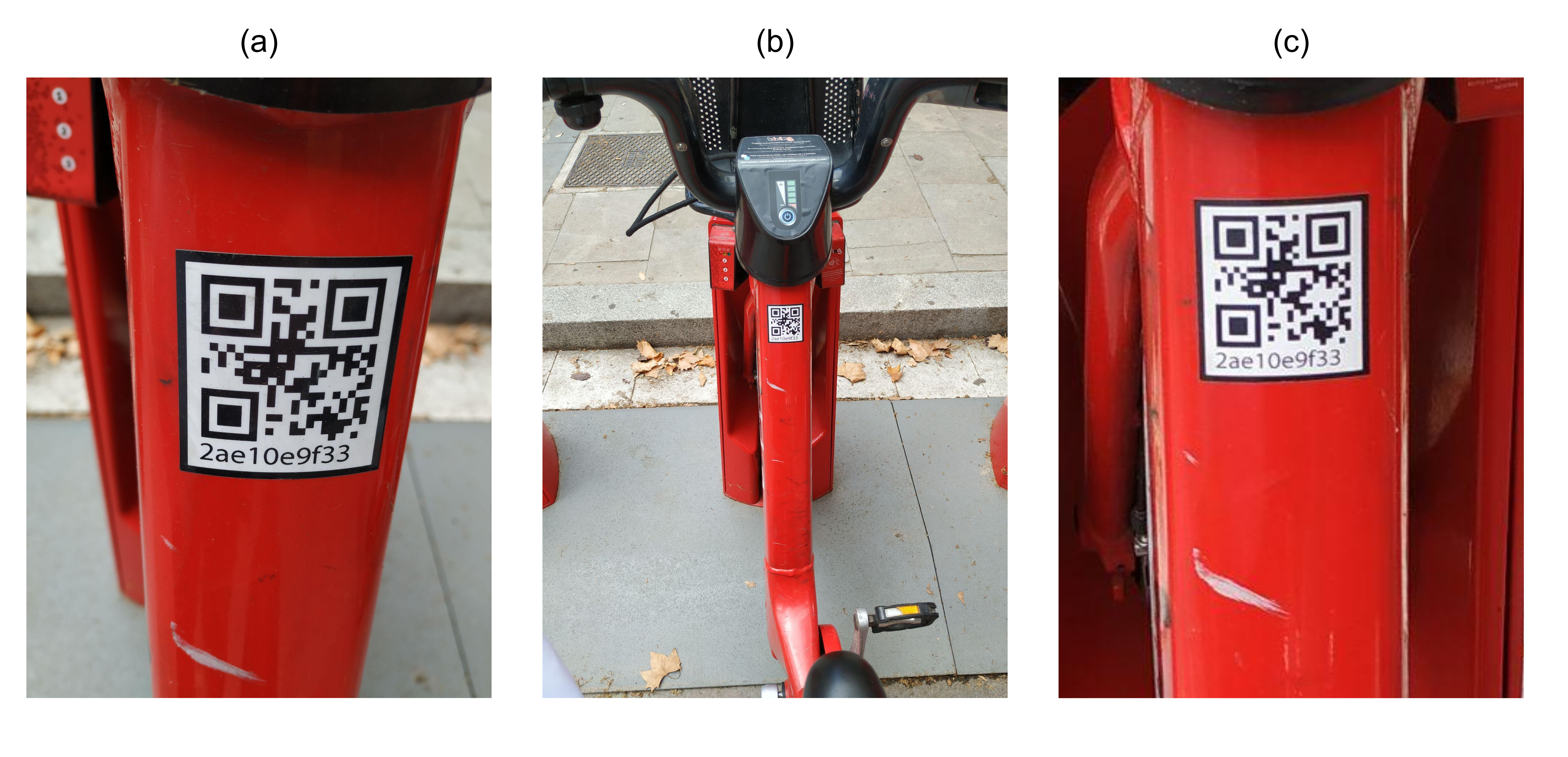
On top of that, in the most common uses, readout is carried out by casual users holding handheld devices (like smartphones) in manifold angles and perspectives. Surprisingly, these perspective effects are not tackled by the original QR Code standard specification, but are so common that are addressed in most of the state-of-the-art QR Code reader implementations [59], [98], [100]. Still, the issues caused by a non-flat topography remain mostly unsolved, and the usual recommendation is just acquiring the QR Code image from a farther distance, where curvature effects turn apparently smaller thanks to the laws of perspective (see [fig:qrcodebike].b and [fig:qrcodebike].c.). This however is a stopgap measure rather than a solution, that fails frequently when the surface deformation is too high or the QR Code is too big.
Other authors have already demonstrated that it is possible to use the QR Code itself to fit the surface underneath to a pre-established topography model. These proposals only work well with surfaces that resemble the shape model assumed (e.g. a cylinder, a sphere, etc.) and mitigate the problem just for a limited set of objects and surfaces, for which analytical topography models can be written.
Regarding perspective transformation models, Sun et al. proposed the idea of using these transformations as a way to enhance readability in handheld images from mobile phones [106]. This idea was explored also by Lin and Fuh, showing that their implementation performed better than ZXing [107], a commercial QR Code decoder formerly developed by Google [100]. Concerning cylindrical transformations, Li, X. et al. [108], Lay et al. [109], [110] and Li, K. [111] reported results on QR Codes placed on top of cylinders. More recently, Tanaka introduced the idea of correcting cylindrical deformation using an Image-to-Image Translation Network [112]. Finally, the problem of arbitrary surface deformations has just been explored very recently. Huo et al. suggested a solution based on Back-Propagation Neural Networks [113]. Kikuchi et al. presented a radically different approach from the standpoint of additive manufacturing by 3D printing the QR codes inside those arbitrary surfaces, and thus solving the inverse problem by rendering apparent planar QR Codes during capture [114].
Here, since a general solution for the decoding of QR Codes placed on top of arbitrary topographies is missing, we present our proposal on this matter based on the thin-plate spline 2D transformation [115]. Thin-plate splines (TPS) are a common solution to fit arbitrary data and have been used before in pattern recognition problems: Bazen et al. [116] and Ross et al. [117] used TPS to match fingerprints; Shi et al. used TPS together with Spatial Transformer Networks to improve handwritten character recognition by correcting arbitrary deformations [118], and Yang et al. reviewed the usage of different TPS derivations in the point set registration problem [119].
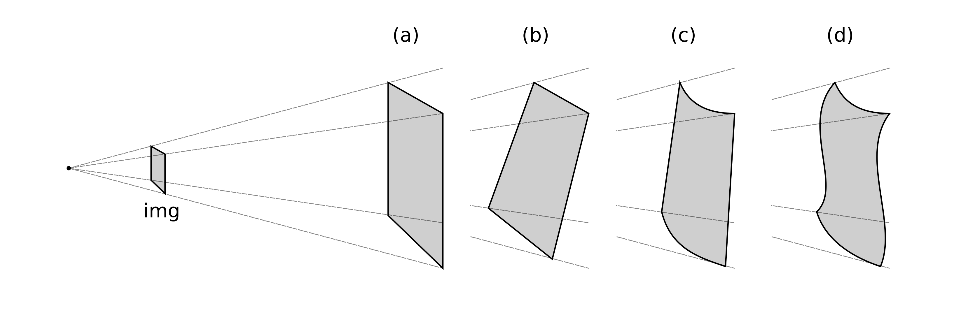
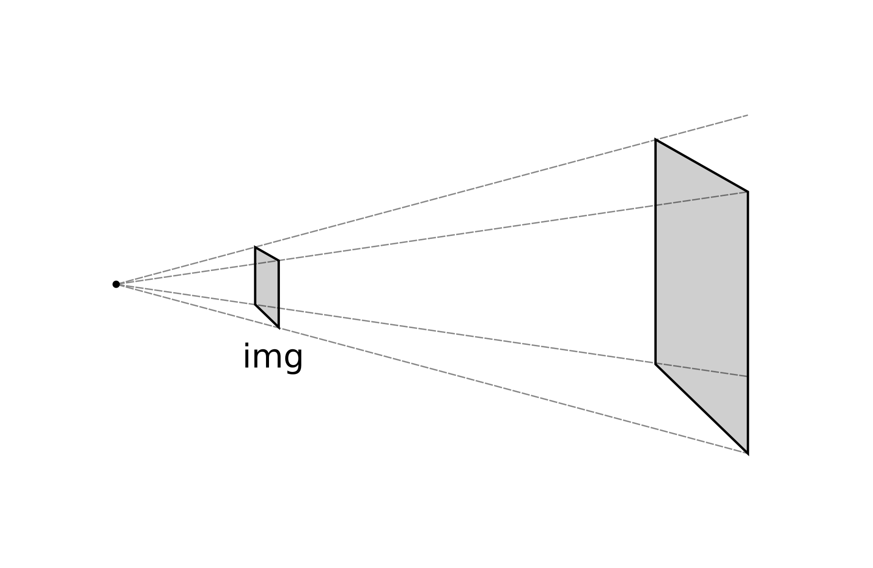
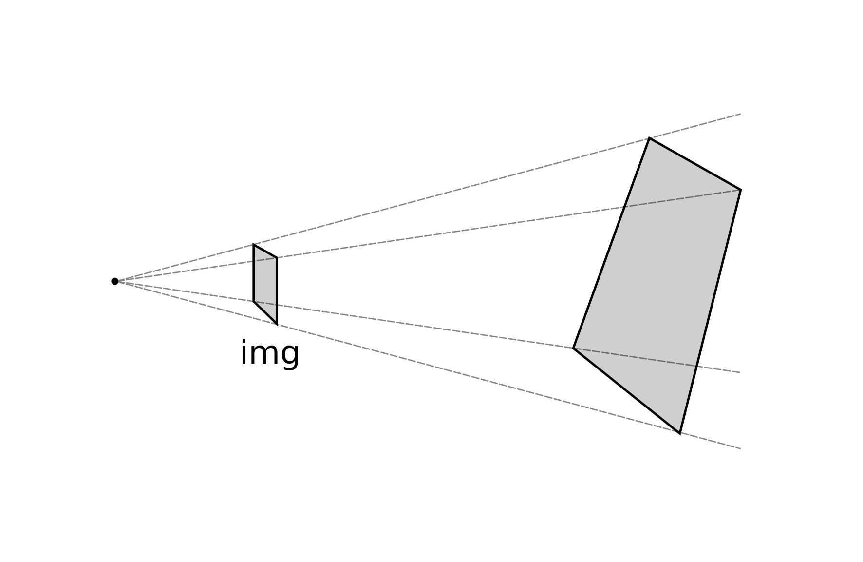
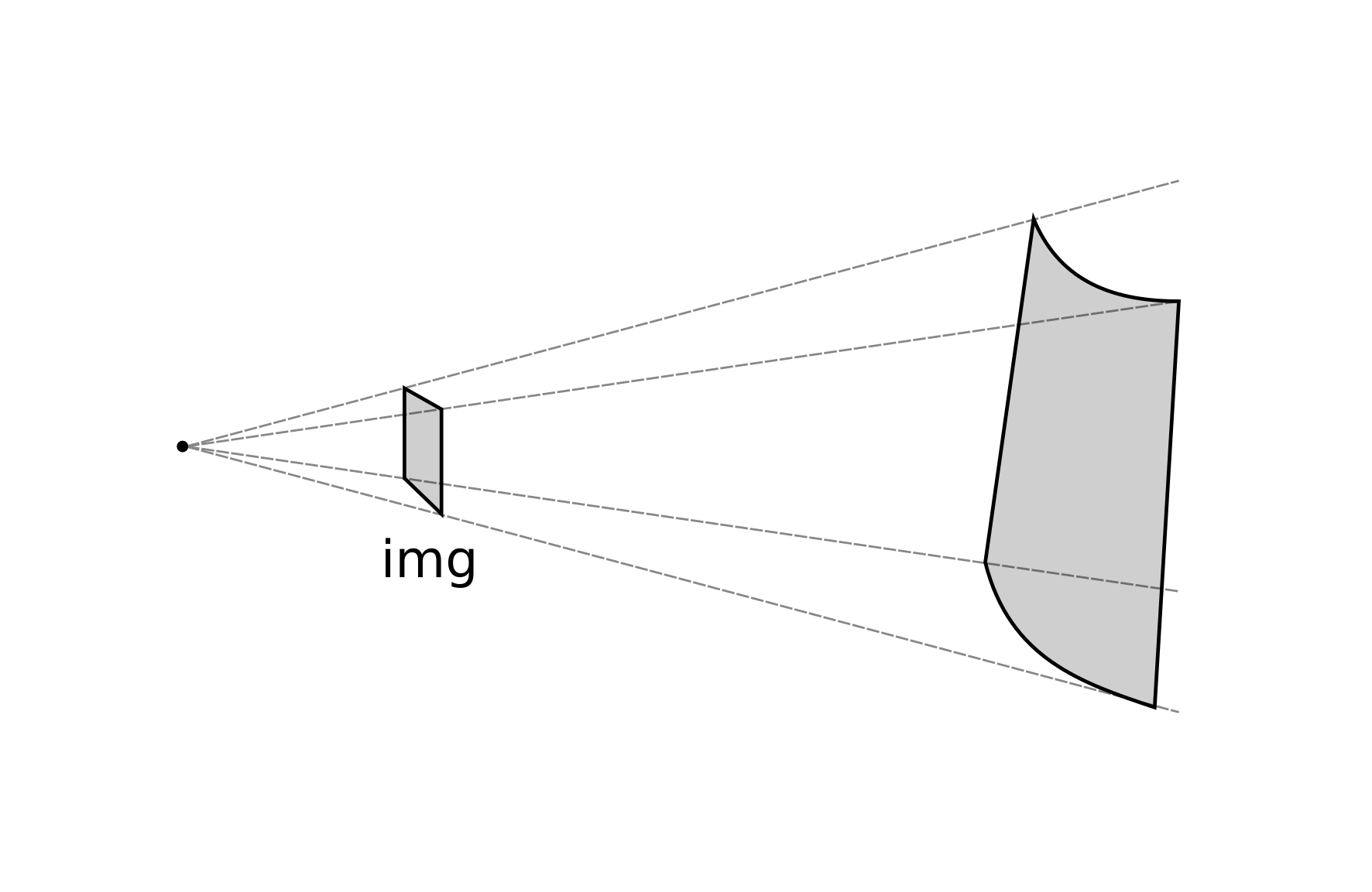
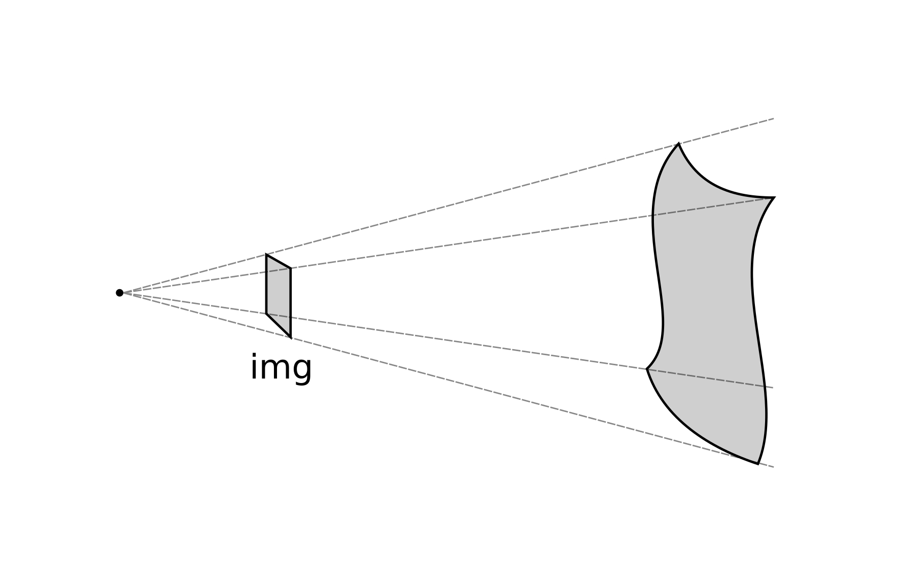
In order to investigate the advantages of the TPS with respect to former approaches, we take here the above-mentioned geometric surface fittings as reference cases, namely: (i) affine coplanar transformations (see [fig:projections].a), (ii) projective transformations (see [fig:projections].b), and (iii) cylindrical transformations (see [fig:projections].c).
Then we introduce our proposal for arbitrary surfaces based on (iv) the thin-plate spline 2D transformation (see [fig:projections].d) and benchmark against each other. With all four methods we use a commercial barcode scanner, ZBar [98], to decode the corrected image and observe the impact of each methodology, not just on the geometrical correction but also on the actual data extraction.
In [ch:3] we have defined images as mappings from an \(\mathbb{R}^2\) plane to a scalar field \(\mathbb{R}\), assuming they are grayscale. [fig:projections] shows this \(\mathbb{R}^2\) plane and labels it as img. Let us define a projective transformation of this plane as an application between two planes:
\[f: \mathbb{R}^2 \to \mathbb{R}^2\].
Also, let the points \((x,y) \in \mathbb{R}^2\) and \((x', y') \in \mathbb{R}^2\), we can then define an analytical projective mapping between those two points as:
\[\label{eq:projectionsmap} \begin{split} x' = f_x (x, y) = a_{0,0} \cdot x + a_{0,1} \cdot y + a_{0,2} \\ y' = f_y (x, y) = a_{1,0} \cdot x + a_{1,1} \cdot y + a_{1,2} \end{split}\]
where \(a_{i,j} \in \mathbb{R}\) are the weights of the projective transform. For a more compact notation, \((x, y)\) and \((x', y')\) can be replaced by homogeneous coordinates [120] \((p_0, p_1, p_2) \in {\rm P}^2 \mathbb{R}\) and \((q_0, q_1, q_2) \in {\rm P}^2 \mathbb{R}\), respectively, that allow expressing the transformation in a full matrix notation3:
\[\label{eq:projectionmatrix} \begin{pmatrix} a_{0,0} & a_{0,1} & a_{0,2} \\ a_{1,0} & a_{1,1} & a_{1,2} \\ a_{2,0} & a_{2,1} & 1 \end{pmatrix} \cdot \begin{pmatrix} p_{0} \\ p_{1} \\ 1 \end{pmatrix} = \begin{pmatrix} q_{0} \\ q_{1} \\ 1 \end{pmatrix}\]
Finally, we can simplify this expression by naming our matrices as:
\[\label{eq:projectionproduct} \mathbf{A} \cdot \mathbf{P} = \mathbf{Q}\]
Here, we will work with four projective transformations: the affine transformation (AFF), the projective transformation (PRO), the cylindrical transformation (CYL) and the thin-plate spline transformation (TPS). We can define all of them as subsets or extensions of projective transformations, so we will have to specifically formulate \(\mathbf{A}\) for each one of them. To do so, we need to know the landmarks in the captured image (acting as vector \(\mathbf{Q}\)) and their “correct” location in a non-deformed corrected image (acting as vector \(\mathbf{P}\)).
Affine (AFF). This transformation uses the landmarks to fit a coplanar plane to the capturing device sensor (see [fig:projections_affine]). It can accommodate translation, rotation, zoom and shear deformations [120]. An affine transformation can be expressed in terms of [eq:projectionmatrix], only taking \(a_{2,0} = a_{2,1} = 0\):
\[\label{eq:projectionmatrix_affine} \begin{pmatrix} a_{0,0} & a_{0,1} & a_{0,2} \\ a_{1,0} & a_{1,1} & a_{1,2} \\ 0 & 0 & 1 \end{pmatrix} \cdot \begin{pmatrix} p_{0} \\ p_{1} \\ 1 \end{pmatrix} = \begin{pmatrix} q_{0} \\ q_{1} \\ 1 \end{pmatrix}\]
This yields to a system with only 6 unknown \(a_{i, j}\) weights. Thus, if we can map at least 3 points in the QR Code surface to a known location (e.g. finder pattern centers) we can solve the system for all \(a_{i, j}\) using the expression of [eq:projectionproduct] with:
\[\begin{split} \mathbf{A} &= \begin{pmatrix} a_{0,0} & a_{0,1} & a_{0,2} \\ a_{1,0} & a_{1,1} & a_{1,2} \\ 0 & 0 & 1 \end{pmatrix} , \\ \mathbf{P} &= \begin{pmatrix} p_{0,0} & p_{0,1} & p_{0,2} \\ p_{1,0} & p_{1,1} & p_{1,2} \\ 1 & 1 & 1 \end{pmatrix} \ and \\ \mathbf{Q} &= \begin{pmatrix} q_{0,0} & q_{0,1} & q_{0,2} \\ q_{1,0} & q_{1,1} & q_{1,2} \\ 1 & 1 & 1 \end{pmatrix}. \end{split}\]
Projective (PRO). This transformation uses landmarks to fit a noncoplanar plane to the capturing plane (see [fig:projections_proj]). Projective transformations use [eq:projectionmatrix] without any further simplification. Also, [eq:projectionproduct] is still valid, but now we have up to 8 unknown \(a_{i, j}\) weights to be determined. Therefore, we need at least 4 landmarks to solve the system for \(\mathbf{A}\), then:
\[\begin{split} \mathbf{A} &= \begin{pmatrix} a_{0,0} & a_{0,1} & a_{0,2} \\ a_{1,0} & a_{1,1} & a_{1,2} \\ a_{2,0} & a_{2,1} & 1 \end{pmatrix} , \\ \mathbf{P} &= \begin{pmatrix} p_{0,0} & p_{0,1} & p_{0,2} & p_{0,3} \\ p_{1,0} & p_{1,1} & p_{1,2} & p_{1,3} \\ 1 & 1 & 1 & 1 \end{pmatrix} \ and \\ \mathbf{Q} &= \begin{pmatrix} q_{0,0} & q_{0,1} & q_{0,2} & q_{0,3} \\ q_{1,0} & q_{1,1} & q_{1,2} & q_{1,3} \\ 1 & 1 & 1 & 1 \end{pmatrix}. \end{split}\]
Notice that the four points in must not be collinear three-by-three, if we want the mapping to be invertible [120].
Cylindrical (CYL). This transformation uses landmarks to fit a cylindrical surface, which can be decomposed into a projective transformation and a pure cylindrical deformation (see [fig:projections_cyl]). Thus, the cylindrical transformation extends the projective general transformation ([eq:projectionsmap]) and adds a non-linear term to the projection:
\[\label{eq:projectionmap_cyl} \begin{split} x' = f_x (x, y) = a_{0,0} \cdot x + a_{0,1} \cdot y + a_{0,2} + w_0 \cdot g(x,y) \\ y' = f_y (x, y) = a_{1,0} \cdot x + a_{1,1} \cdot y + a_{1,2} + w_1 \cdot g(x,y) \end{split}\]
where \(g(x, y)\) is the cylindrical term, which takes the form of [108], [111]:
\[g(x, y) = \begin{cases} \sqrt{r^2 - (c_0 - x)^2} & if \ \ r^2 - (c_0 - x)^2 \geq 0 \\ 0 & if \ \ r^2 - (c_0 - x)^2 < 0 \end{cases}\]
where \(r \in \mathbb{R}\) is the radius of the cylinder, and \(c_0 \in \mathbb{R}\) is the first coordinate of any point in the centerline of the cylinder. Now, [eq:projectionmatrix] becomes extended with another dimension for cylindrical transformations:
\[\begin{pmatrix} w_0 & a_{0,0} & a_{0,1} & a_{0,2} \\ w_1 & a_{1,0} & a_{1,1} & a_{1,2}\\ w_2 & a_{2,0} & a_{2,1} & 1 \end{pmatrix} \cdot \begin{pmatrix} g(p_0, p_1) \\ p_{0} \\ p_{1} \\ 1 \end{pmatrix} = \begin{pmatrix} q_{0} \\ q_{1} \\ 1 \end{pmatrix}\]
Applying the same reasoning as before, we have now 8 unknown \(a_{i,j}\) plus 3 unknown \(w_{j}\) weights to fit. Equivalent matrices ([eq:projectionproduct]) for cylindrical transformations need now at least 6 landmarks and look like:
\[\begin{split} \mathbf{A} &= \begin{pmatrix} w_0 & a_{0,0} & a_{0,1} & a_{0,2} \\ w_1 & a_{1,0} & a_{1,1} & a_{1,2} \\ w_2 & a_{2,0} & a_{2,1} & 1 \end{pmatrix} , \\ \mathbf{P} &= \begin{pmatrix} g(p_{0,0}, p_{1,0}) & ... & g(p_{0,5}, p_{1,5}) \\ p_{0,0} & ... & p_{0,5} \\ p_{1,0} & ... & p_{1,5} \\ 1 & ... & 1 \end{pmatrix} \ and \\ \mathbf{Q} &= \begin{pmatrix} q_{0,0} & ... & q_{0,5} \\ q_{1,0} & ... & q_{1,5} \\ 1 & ... & 1 \end{pmatrix}. \end{split}\]
Thin-plate splines (TPS). This transform uses the landmarks as centers of radial basis splines to fit the surface in a non-linear way that resembles the elastic deformation of a metal thin-plate bent around fixed points set at these landmarks [115] (see [fig:projections_tps]). The radial basis functions are real-valued functions:
\[h: [0, \inf) \to \mathbb{R}\]
that take into account a metric on a vector space. Their value only depends on the distance to a reference fixed point:
\[h_c(v) = h(|| v - c ||) \label{eq:tpskernel}\]
where \(v \in \mathbb{R}^n\) is the point in which the function is evaluated, \(c \in \mathbb{R}^n\) is the fixed point, \(h\) is a radial basis function. [eq:tpskernel] reads as "\(h_c(v)\) is a kernel of \(h\) in \(c\) with the metric \(||\cdot||\)". Similarly to cylindrical transformations ([eq:projectionmap_cyl]), we extended the affine transformation ([eq:projectionsmap]) with \(N\) nonlinear spline terms:
\[\begin{split} x' &= f_x (x, y) = a_{0,0} \cdot x + a_{0,1} \cdot y + a_{0,2} + \sum_{k=0}^{N-1} w_{0,k} \cdot h_k ((x, y)) \\ y' &= f_y (x, y) = a_{1,0} \cdot x + a_{1,1} \cdot y + a_{1,2} + \sum_{k=0}^{N-1} w_{1,k} \cdot h_k ((x, y)) \end{split}\]
where \(w_{j,k}\) are the weights of the spline contributions, and \(h_k (x, y)\) are kernels of \(h\) in \(N\) landmark points.
These radial basis function remains open to multiple definitions. Bookstein [115] found that the second order polynomial radial basis function is the proper function to compute splines in \(\mathbb{R}^2\) mappings in order to minimize the bending energy, and mimic the elastic behavior of a metal thin-plate. Thus, let \(h\) be:
\[h(r) = r^2 \ln(r)\]
with the corresponding kernels computed using the euclidean metric:
\[|| (x, y) - (c_x, c_y) || = \sqrt{(x - c_x)^2 + (y - c_y)^2}\]
Finally, in matrix representation, terms from [eq:projectionproduct] are expanded as follows:
\[\begin{split} \mathbf{A} &= \begin{pmatrix} w_{0,0} & ... & w_{0, N-1} & a_{0,0} & a_{0,1} & a_{0,2} \\ w_{1,0} & ... & w_{1,N-1} & a_{1,0} & a_{1,1} & a_{1,2} \end{pmatrix} , \\ \mathbf{P} &= \begin{pmatrix} h_0(p_{0,0}, p_{1,0}) & ... & h_0(p_{0,N-1}, p_{1,N-1}) \\ \vdots & ... & \vdots \\ h_{N-1}(p_{0,0}, p_{1,0}) & ... & h_{N-1}(p_{0,N-1}, p_{1,N-1}) \\ p_{0,0} & ... & p_{0,N-1} \\ p_{1,0} & ... & p_{1,N-1} \\ 1 & ... & 1 \end{pmatrix} \ and \\ \mathbf{Q} &= \begin{pmatrix} q_{0,0} & ... & q_{0,N-1} \\ q_{1,0} & ... & q_{1,N} \end{pmatrix}. \end{split} \label{eq:qr_tps_APQ}\]
First, notice that only \(a_{i,j}\) affine weights are present, since this definition does not include a perspective transformation. Second, in contrast with previous transformations, this system is unbalanced: we have a total of \(2N + 6\) weights to compute (\(2N\) \(w_{j,k}\) spline weights plus 6 \(a_{i,j}\) affine weights), however, we only have defined \(N\) landmarks.
In the previous transformations, we used additional landmarks to solve the system, but Bookstein imposed an additional condition of the spline contributions: the sum of \(w_{j,k}\) coefficients to be \(\mathrm{0}\), and also their cross-product with the \(p_{i,k}\) landmark coordinates [115]. With such a condition, spline contributions tend to \(\mathrm{0}\) at infinity, while affine contributions prevail. This makes our system of equations solvable and can be expressed as:
\[\begin{pmatrix} w_{0,0} & ... & w_{0, N-1} \\ w_{1,0} & ... & w_{1,N-1} \end{pmatrix} \cdot \begin{pmatrix} p_{0,0} & ... & p_{0,N-1} \\ p_{1,0} & ... & p_{1,N-1} \\ 1 & ... & 1 \end{pmatrix}^T = 0\]
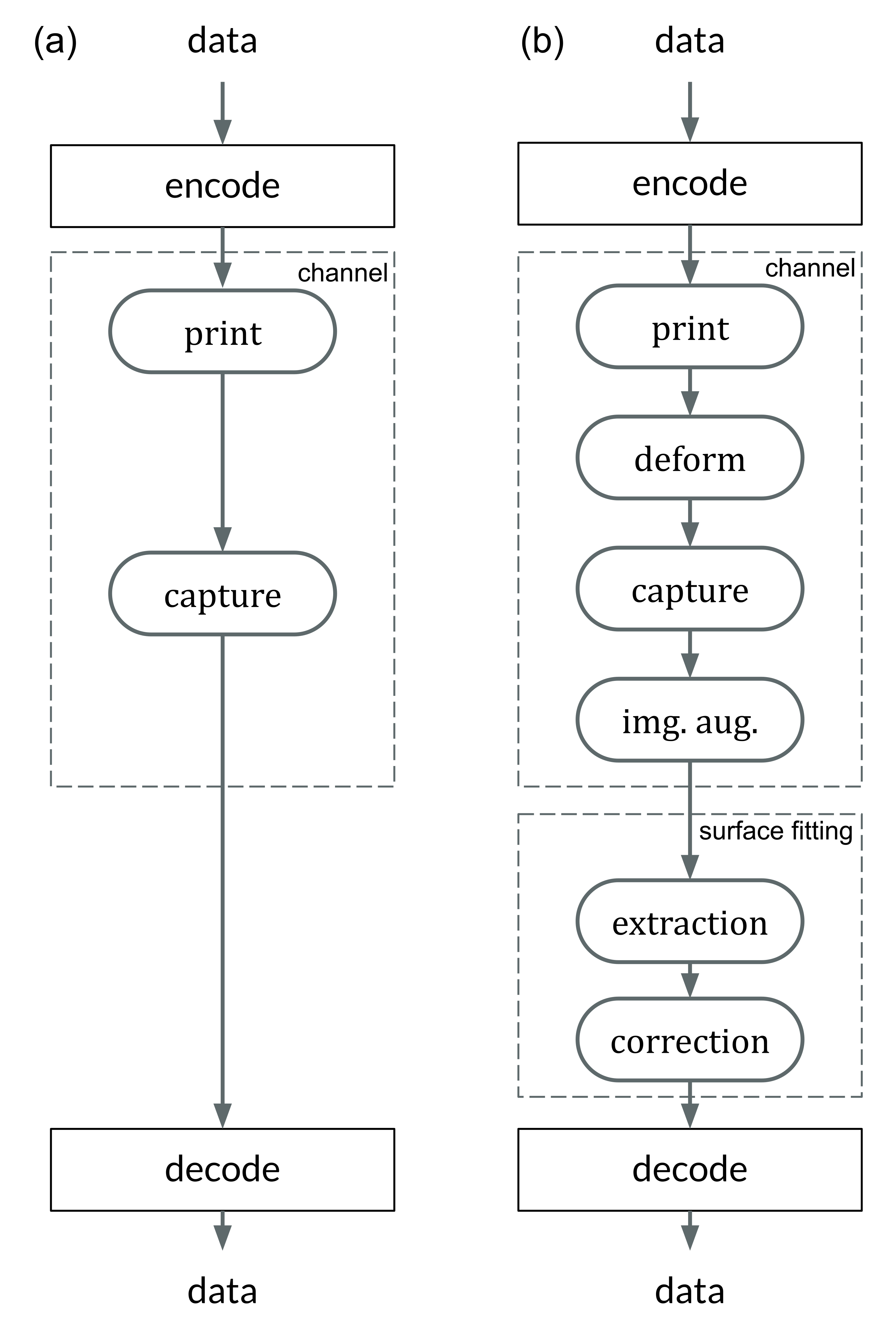
Experiments were designed to reproduce the QR Code life-cycle in different scenarios, which can be regarded as a digital communication channel: a message made of several bytes with their corresponding error correction blocks is encoded in the black and white pixels of the QR Code, that is transmitted through a visual channel (i.e. first displayed or printed and then captured by a camera), and finally decoded, and the original message retrieved (see [fig:pipeline].a).
In this context, the effects of the challenging surface topographies can be seen as an additional step in the channel, where the image is deformed in different ways prior to the capture. To investigate these effects we attached our QR codes to real complex objects to collect pictures with relevant deformations (see details below). Then, in order to expand our dataset, we incorporated an image augmentation step that programmatically added additional random projective deformations to the captured images [121]. Finally, we considered the surface fitting and correction as an additional step in the QR Code processing workflow, prior to attempting decoding. This proved more effective than directly attempting the QR Code decoding based on the distorted image with deformed position and feature patterns due to the surface topography (see [fig:pipeline].b).
We created 3 datasets to evaluate the performance of different transformations in different scenarios with arbitrary surface shapes.
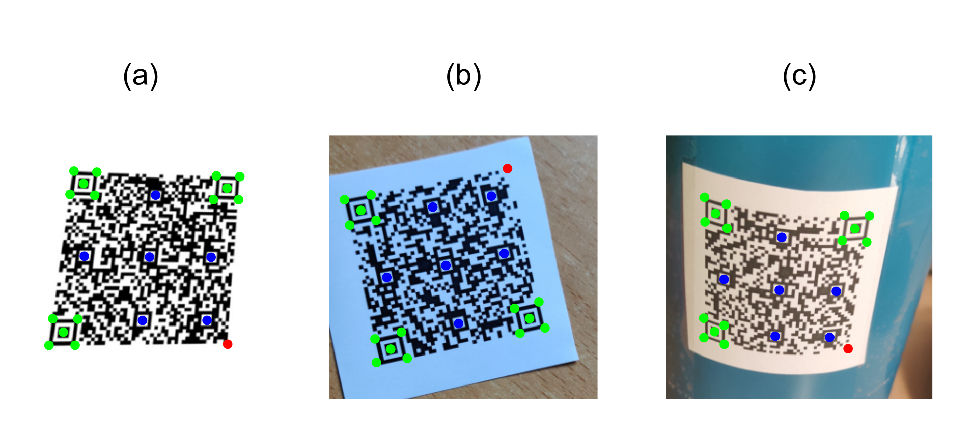
Synthetic QR Codes (SYNT). This dataset was intended to evaluate the impact of data and geometry of the QR Code on the proposed deformation correction methods. To that end, we generated the QR Codes as digital images, without printing them, and applied to them affine and projective transformations directly with image augmentation techniques (see [fig:datasetexamples].a). This dataset contained 12 QR Code versions (from version 1 to 12), each of them repeated 3 times with different random data (IDs), and 19 augmented images plus the original one. The mutual combination of all these variations yielded a total of 720 images to be processed by the proposed transformations (see [tab:datasets]).
QR Codes on flat surfaces (FLAT). In this dataset, we only encoded 1 QR Code version 7 and printed it. We placed this QR Code on different flat surfaces and captured images (see [fig:datasetexamples].b). Thus, we only expected projective deformations in this dataset, to be used as a reference. We also augmented the captured images to match the same quantity of images from the previous dataset (see [tab:datasets]).
QR Codes on challenging surfaces (SURF). In this dataset, we used the same QR Code we used in the FLAT dataset, but placed on top of challenging surfaces, such as bottles, or manually deforming the QR Codes (see [fig:datasetexamples].c). We expected here to have cylindrical and arbitrary deformations in the dataset. Also, we augmented the captured images to match the size of the other datasets (see [tab:datasets]).
For all the datasets, the same features were extracted: finder patterns, alignment patterns and the fourth corner, see for more details about the extraction of those features in [ch:3].
| SYNT | Values | Dataset size |
|---|---|---|
| Version | from 1 to 13 | 12 |
| IDs (per version) | random | 3 |
| Captures | 1 | |
| Image augmentation | 20 | |
| Total | 720 | |
| FLAT | Values | Dataset size |
| Version | 7 | 1 |
| IDs (per version) | https://color-sensing.com/ | 1 |
| Captures | 48 | |
| Image augmentation | 15 | |
| Total | 720 | |
| SURF | Values | Dataset size |
| Version | 7 | 1 |
| IDs (per version) | https://color-sensing.com/ | 1 |
| Captures | 48 | |
| Image augmentation | 15 | |
| Total | 720 |
We fitted the four transformations (AFF, PRO, CYL and TPS) to the surface underneath all the QR Code samples from the three datasets (SYNT, FLAT and SURF). To evaluate visually how accurate each transformation was, a squared lattice of equally spaced points on the predicted QR Code surface was back-projected into the original image space. For illustration purposes, results on representative samples of the SYNT, FLAT and SURF datasets can be seen in [fig:resultsSYNT], [fig:resultsFLAT] and [fig:resultsSURF], respectively.
Our first dataset, SYNT, contained samples with affine ([fig:resultsSYNT].a) and projective ([fig:resultsSYNT].b) deformations. We observed that all four transformations achieved good qualitative fittings with images presenting affine deformations. This is an expected result, since all transformations implement affirm terms. Consequently, when it comes to projective deformations, the AFF transformation failed to adjust the fourth corner (the one without any finder pattern, see [fig:qrcodeparts].a), as expected. Comparatively, the PRO and the CYL transformations lead to similarly good results, since both can accommodate perspective effects. Finally, TPS fitted the surface well, specially inside the QR Code, and a slight non-linear deformation was present outside the boundaries of the barcode, but these are irrelevant for QR Code decoding purposes.
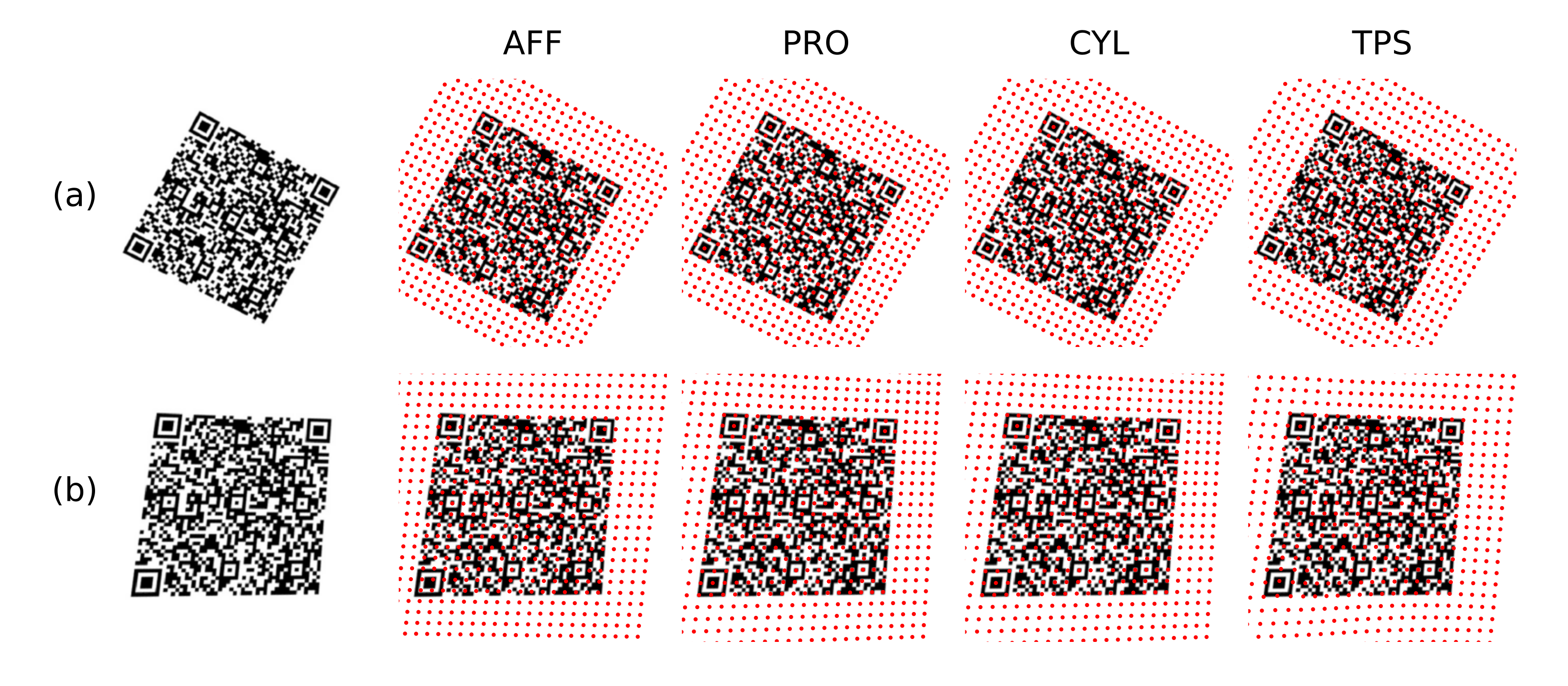
The FLAT dataset involved QR Codes that were actually printed and then imaged with a smartphone camera. These QR Codes were captured in projective deformations ([fig:resultsFLAT].b), some of them resembling affine deformations ([fig:resultsFLAT].a), and most of them just a combination of both. Qualitative performance comparison is similar to that of the SYNT dataset. Again, the AFF transformation failed to correctly approach the fourth corner. Also, we confirmed that PRO, CYL and TPS performed well for the FLAT images, but TPS showed a non-linear, irrelevant, overcorrection outside the barcode.
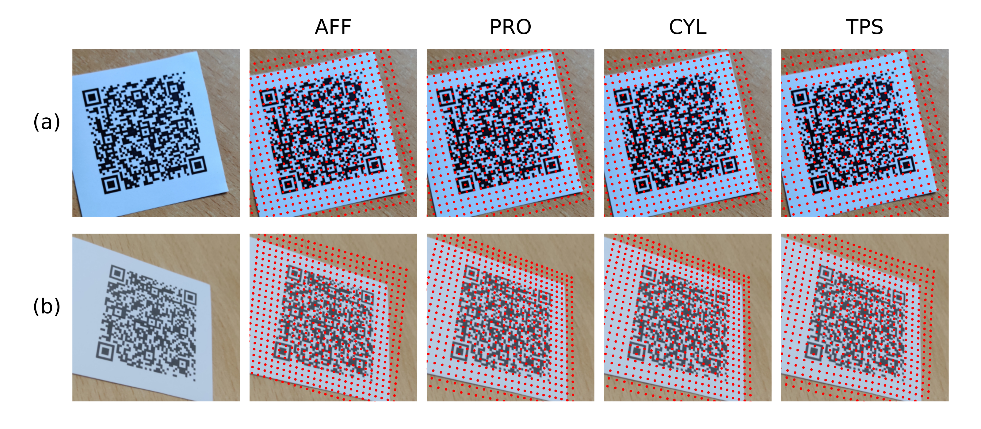
The SURF dataset was the most challenging dataset in terms of modeling adverse surface topographies. QR Codes here were imaged again with a smartphone, but in this case the surface under the barcode was distorted in several ways: randomly deformed by hand ([fig:resultsSURF].a), placed on top of a small bottle ([fig:resultsSURF].b), a large bottle ([fig:resultsSURF].c), etc. Results showed that AFF, PRO and CYL methods were not able to correctly match a random surface (i.e. deformed by hand), as expected. Instead, TPS worked well in these conditions, being a great example of the power of the spline decomposition to match slow varying topographies, if a sufficiently high number of landmarks is available. For cylindrical deformations (i.e. QR Codes in bottles), AFF and PRO methods were again unsuccessful. CYL performed better with the small bottles than with the large ones. Apparently, higher curvatures (i.e. lower bottle radius \(r\)) facilitate the fitting of this parameter and improve the quality of the overall prediction radius of the projected cylinder before fitting the surface. Thus, the CYL method properly fits the cylinder radius from one of the sides of the QR Codes with 2 finder patterns and often fails to fit the opposite side. Interestingly, The TPS method performed opposite to the CYL method in the cylindrical deformations, tackling better surfaces with mild curvatures.
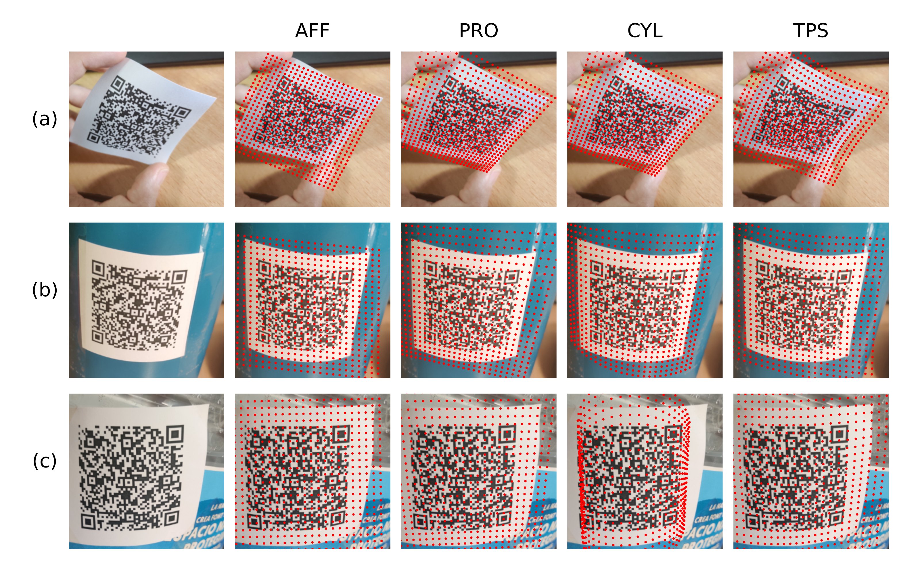
In order to evaluate the impact of these surface prediction capabilities on the actual reading of the QR Code data, we run the full decoding pipeline mentioned in [fig:pipeline] for all the images in the three datasets (SYNT, FLAT and SURF) with the four transformations (AFF, PRO, CYL and TPS). There, once surface deformation was corrected, the QR Code data was extracted with one of the most widespread barcode decoder (ZBar [56], [122]). Therefore, in this experiment we are actually evaluating how the error made on the assessment of the QR Code geometry, due to surface and perspective deformations, impacts on the evaluation of the individual black/white pixel bits; and to what extent the native QR Code error correction blocks (based on Reed-Solomon according to the standard) can revert the errors made. We then defined a success metric of data readability[25] (\(\mathcal{R}\)) as:
\[\mathcal{R} = 100 \cdot \frac{N_{decoded}}{N_{total}} [\%]\]
where \(N_{decoded}\) is the number of QR Codes successfully decoded and \(N_{total}\) is the total amount of QR Codes of a given dataset and transformation. Such a number has a direct connection with the user experience. In a manual reading scenario, it tells us how often the user will have to repeat the picture (e.g. \(\mathcal{R} = 95 \%\) means 5 repetitions out of every 100 uses). In applications with automated QR Code scanning, this measures how long it will take to pick up the data.
[fig:readability_dataset] summarizes the readability performance of the four transformations with the three datasets. For the SYNT and FLAT datasets, PRO, CYL and TPS scored 100% or close. AFF scored only 78% and 60% for the SYNT and the FLAT datasets, respectively. This is because AFF lacks the perspective components that PRO and CYL incorporate to address this problem. It is noteworthy that the TPS scored similar to the PRO and CYL for these two datasets: despite TPS does not include perspective directly, it is composed of affine and non-linear terms, and the later ones can fit a perspective deformation.
This behavior is also confirmed for the segregated data on the SYNT dataset (see [fig:readability_SYNT]), where the TPS performed slightly worse on images with a perspective deformation, similarly to the AFF. Also in [fig:readability_SYNT], we see that AFF showed its best performance (97%) in the subset of images where only affine transformation was present, rendering lower in the projective ones (70%).
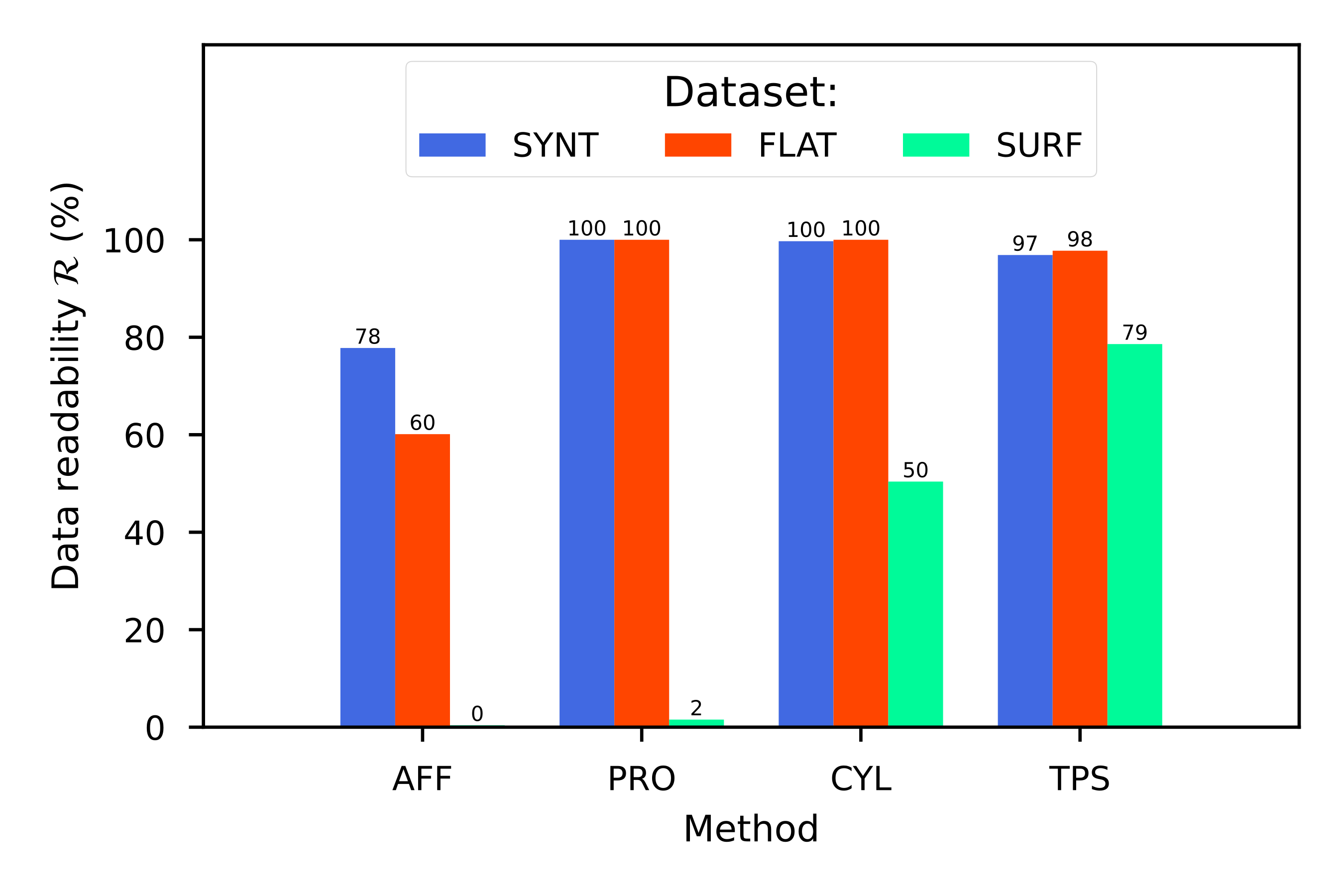
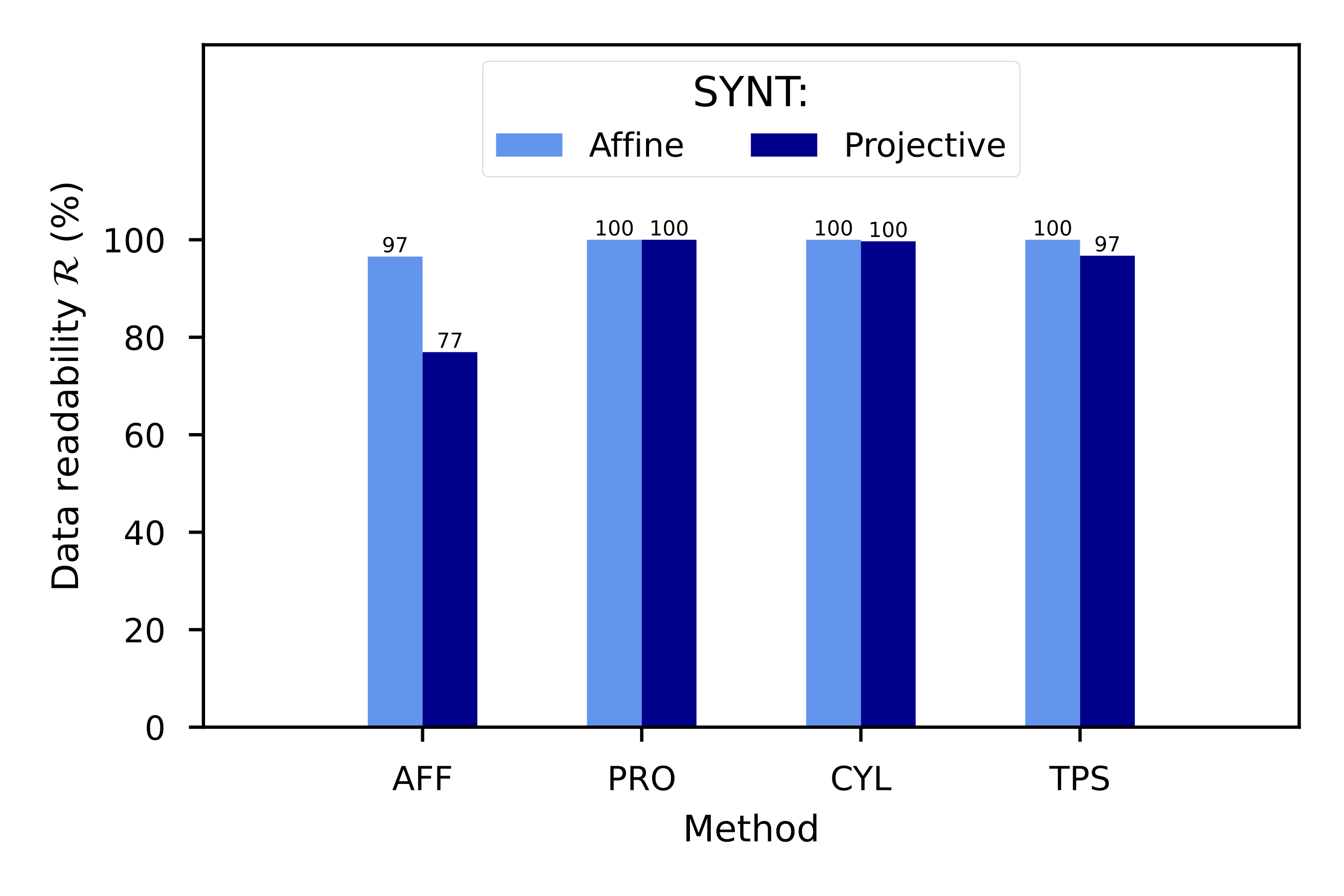

[fig:readability_SURF] shows the segregated data for the SURF dataset, neither the AFF nor the PRO transformations decoded almost any QR Code (1%-2%). CYL performed well for cylindrical surfaces in the SURF dataset (62%), but got beaten by the TPS results by 13 points (from 62% to 75%). Moreover, CYL scored less than 30% in images without explicit cylindrical deformations, as expected; while the TPS remained well over 85%. This is a remarkable result for the TPS, considering that the rest of transformations failed completely at this task.
Finally, we wanted to benchmark the methodology proposed here with a popular, state-of-the-art decoder like ZBar. To that end, we fed ZBar with all our datasets of images (without pre-processing and with surface geometry corrections made). [fig:readability_ZBAR] shows that the ZBar implementation (consisting of reading QR Code pixels out of reading each line of the QR Code as one dimensional barcode[98]) performs very well with the SYNT dataset. But, in the more realistic smartphone-captured images from FLAT, ZBar performed poorly, succeeding only in approximately in of the dataset.
Surprisingly, ZBar was still able to decode some SURF dataset images. We compared these results with a combined sequence of CYL and TPS transformations that can be regarded as TPS with a fall-back to the CYL method, since CYL has its own fall-back into PRO. Our solution, improved the good results of ZBar in the SYNT dataset, obtained a perfect score in the FLAT dataset where ZBar struggles (100% vs 75%), and displayed a remarkable advantage (84% vs 19%) in decoding the most complex SURF dataset. We can therefore state that the here-proposed methodology outperforms the state-of-the-art when facing complex surface topographies.
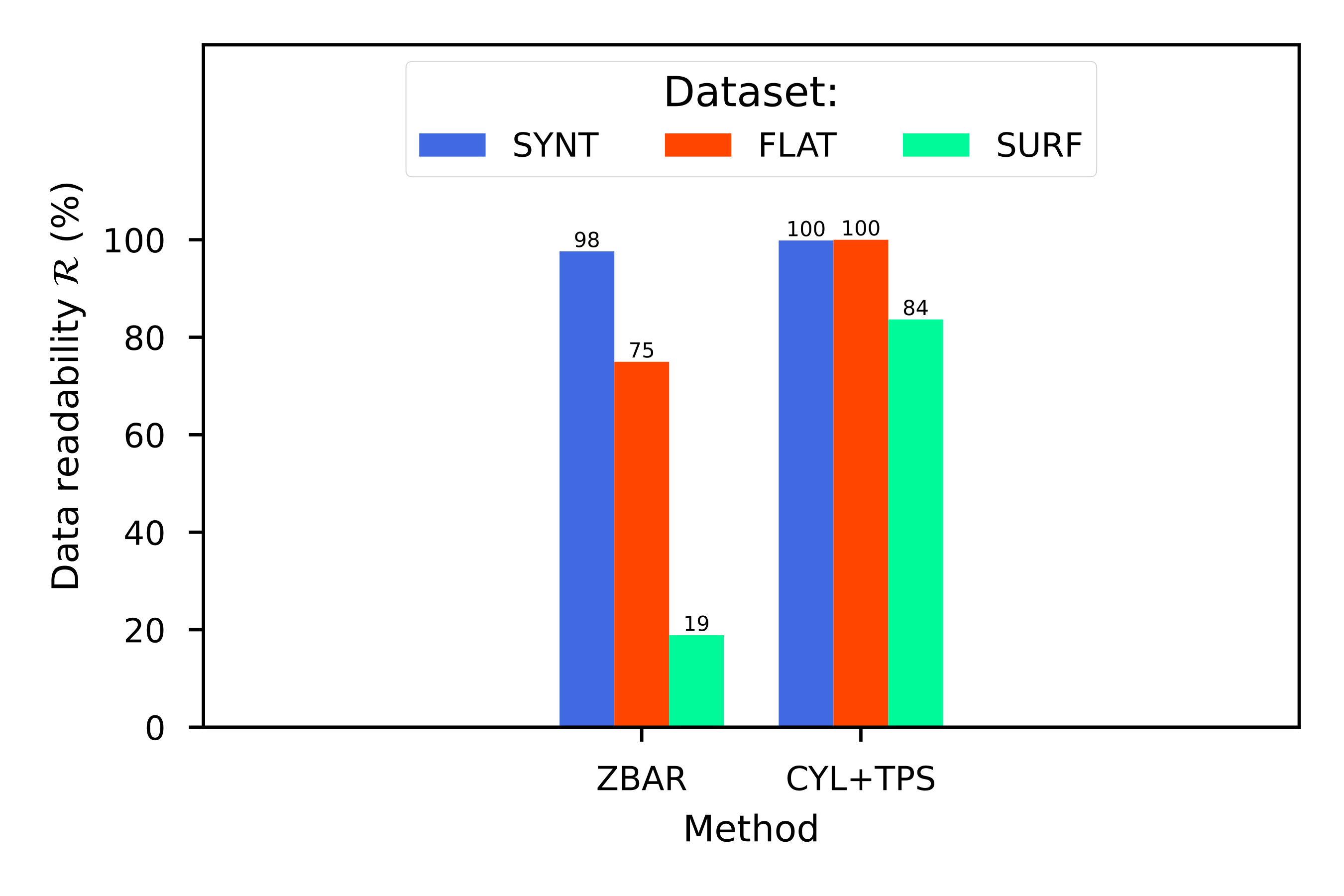
We have presented a method to increase the readout performance of QR Codes suffering surface deformations that challenge the existing solutions. The thin-plate splines (TPS) transformation has proven to be a general solution for arbitrary deformations that outperforms other transformations proposed in the literature (AFF, PRO, CYL), and the commercial implementation ZBar, by more than 4 times.
TPS presented a few corner cases when approaching high perspective projective transformations (i.e. the QR Code is way noncoplanar with the capture device in a flat surface), where CYL and PRO methods performed very well. The results presented here point at an optimum solution based on a sequential combination of the three methods as fall-back alternatives (i.e. TPS → CYL → PRO).
This work has demonstrated how the TPS method is a suitable candidate to correct images where QR Codes are present using traditional feature extraction of the QR Codes features themselves. Futures developments could involve enhancements to this methodology, and we expose now some ideas.
First, one could enhance the TPS definition to incorporate perspective components into the TPS fittings, which one of the differences between the CYL and the TPS method. This was done by Bartoli et al. [123]. In their work they renamed the TPS method as DA-Warp, standing for ’Deformable Affine Warp’, and introduced three new methods: the RA-Warp – ’Rigid Affine Warp’ –, the DP-Warp – ’Deformable Perspective Warp’ – and the RP-Warp – ’Rigid Perspective Warp’ –. Their framework could be applied to images with QR Codes to increase the performance of our solution and avoid the fall-back TPS → CYL → PRO.
Second, approximating the radial basis contributions to the TPS fittings is a well-know technique to relax the condition that each landmark must be mapped directly to its respective landmark in the corrected image [124], [125]. This is usually done by adding a smoothing factor \(\lambda\) to the diagonal of the \(\textbf{P}\) array (see [eq:qr_tps_APQ]). We deepen in this methodology in [ch:6] when we applied TPS to color correction. For QR Code extraction we discarded to use it because we often want the extracted key features to match exactly their position in the recovered image. Nevertheless, as it was not checked experimentally it should be addressed in some future work.
Third, in this work we demonstrated that TPS can be used to map the surface where the QR Code is posed, no matter how adversarial that surface was – provided it is continuous and derivable –. The TPS framework needs a huge quantity of landmark points to compute the TPS correction, the more, the better. We extracted these landmarks with classical feature extractors (contour detection, pattern matching, etc.), but one could use neural networks to solve that problem. For example, Shi et al. [118] presented an interesting solution which also involved TPS. They trained a neural network to discover the optimal landmarks for a given image with a text, in order to rectify it using a TPS method, and later on, apply a text recognition network to recover the text. Other authors, like Li et al. [126] have presented recent work using the popular general-purpose recognition neural network ’YOLOv3’ [127] to locate the corners of ArUco codes [19].
Finally, our method could be applied to other 2D barcodes, such as DataMatrix, Aztec Code or MaxiCode. The main blocker to implement our methodology to such machine-readable patterns is the feature extraction. For example, QR Codes implement a variety of patterns, as detailed in [ch:3]: finder, alignment and timing patterns. Instead, DataMatrix codes only present timing patterns [46]. But perhaps this handicap might be avoided using better extractors that use the Hough transform to recover the full grid of the machine-readable pattern not only the key features [128].
As previously stated, the popularization of digital cameras enabled an easier access to photography devices to the people. Nowadays, modern smartphones have onboard digital cameras that can feature good color reproduction for imaging uses. However, when actual colorimetry is needed, the smartphone camera sensor does not suffice, needing auxiliary ad hoc tools to evaluate color and guarantee image consistency among datasets [129].
As we have introduced in [ch:3], a traditional approach to achieve a general purpose color calibration is the use of color correction charts, introduced by C.S. McCamy et. al. in 1976 [13], combined with color correction techniques. It is safe to say that, in most of these post-capture color correction techniques, increasing the number and quality of the color references offers a systematic path towards better color calibration. We pursue this idea further in next [ch:6].
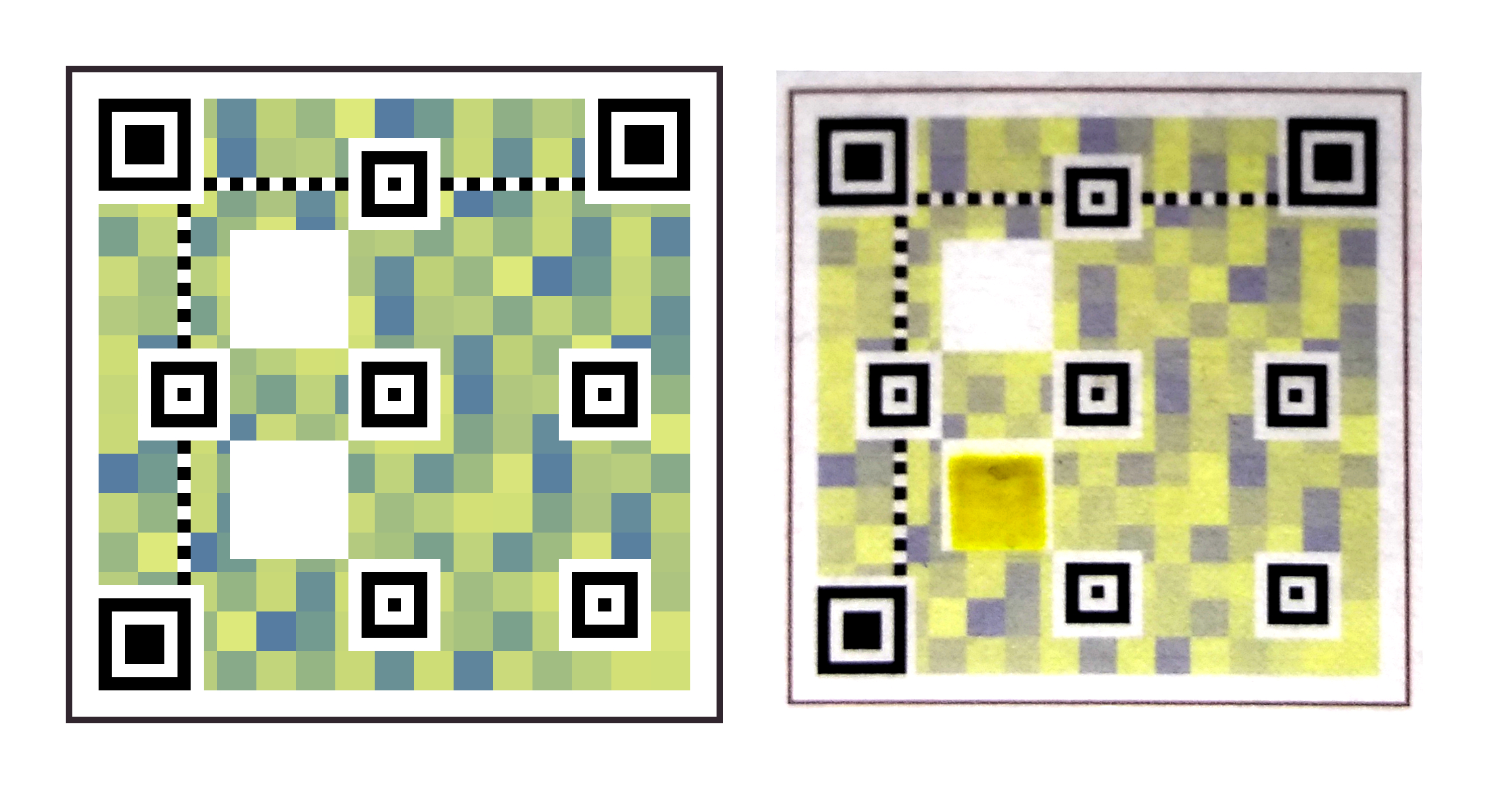
In 2018, we presented a first implementation of a machine-readable pattern (see [fig:machinereadable2018]), based on the image recognizable structures of the QR Codes, that integrated a color changing indicator (sensitive to gases related to bad odor) and a set of color references (to measure that color indication) [29]. In 2020, we reported a more refined solution allocating hundreds of colors into another machine-readable pattern, suitable to measure multiple gas sensors by means of color changes, alongside with the reference colors inside a pseudo QR Code pattern [30]. In both solutions, the QR Code finder, the timing and the alignment patterns (detailed in [ch:3]) were present and used to find, locate and sample the gas sensitive pixels and the reference colors, but all the digital information was removed. These were, therefore, ad hoc solutions that lacked the advantages of combining a compact colorimetric readout and calibration pattern with the digital data available in a QR Code. These solutions are presented [ch:7] from the standpoint of colorimetric sensors in.
Linking the colorimetric problem to a set of digital information opens the door to many potential uses related to automation. For example, the digital data could store a unique ID to identify the actual color calibration references used in the image, or other color-measurement properties e.g. by pointing at a data storage location. When used, for example, in smart packaging, this enables the identification of each package individually, gathering much more refined and granular information.
In this chapter, we propose a solution for that, by placing altogether digital information and color references without breaking the QR Code standard in a back-compatible Color QR Code implementation for colorimetric applications. Our solution modifies the above-presented default QR Code encoding process (see [fig:defaultqrflow]), to enhance the QR Code to embed colors in a back-compatible way (see [fig:colorqrflow]).
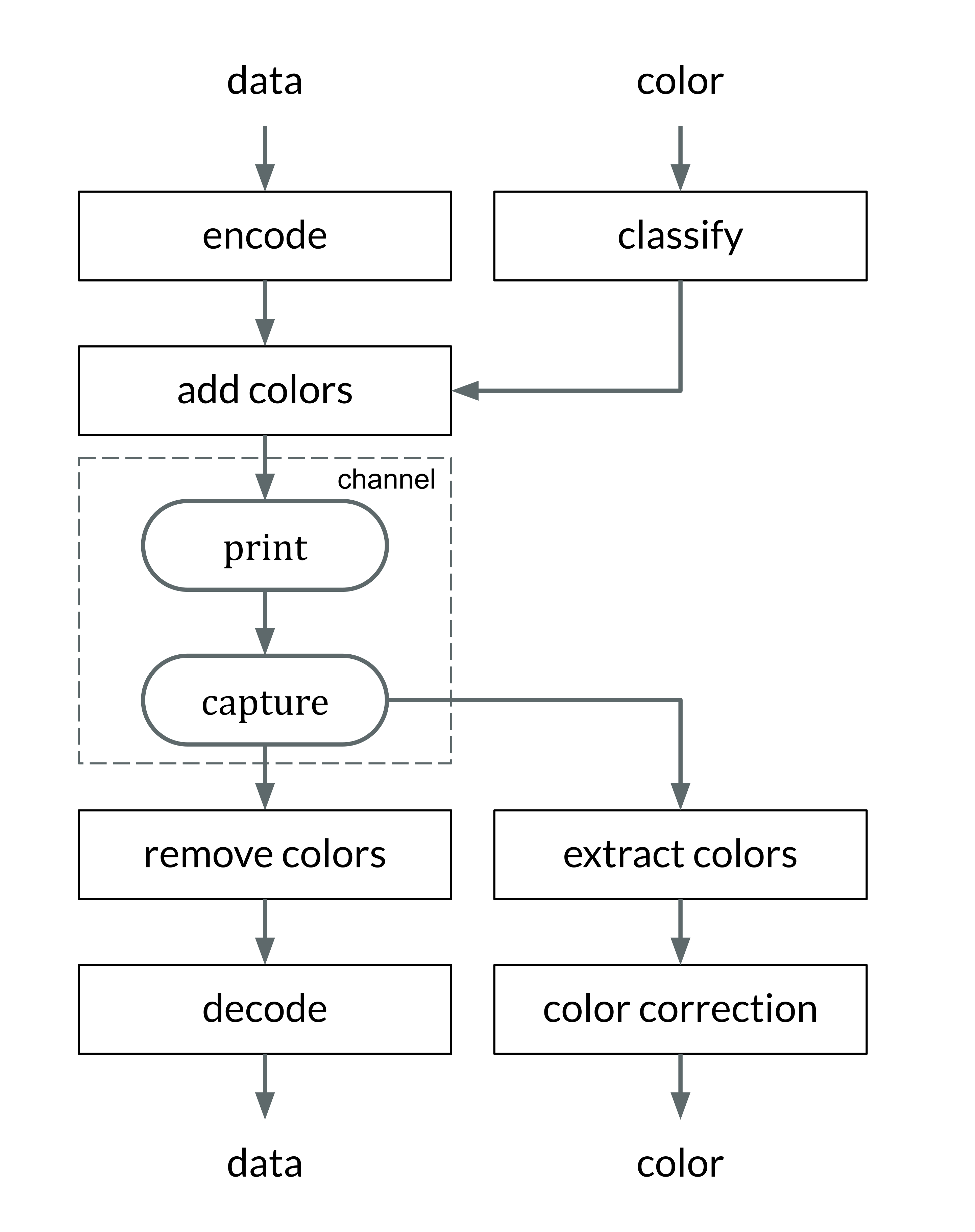
This solution is inspired by, but not directly based on, previous Color QR Codes proposals that aimed at enhancing the data storage capacity of a QR Code by replacing black and white binary pixels by color ones (see [fig:othercolorqrs]) [57], [130]–[132]. Those approaches offer non-back-compatible barcodes that cannot be decoded with standard readers. Instead, our work offers a design fully compatible with conventional QR Codes. Evidently, without a specialized reader, the color calibration process cannot be carried out either, but back-compatibility assures that any standard decoder will be able to extract the digital data to, e.g. point at the appropriate reader software to carry out the color correction in full. From the point of view of the usability, back-compatibility is key to enable a seamless deployment of this new approach to color calibration, using only the resources already available in smartphones (i.e. the camera and a standard QR decoder).
![Previous state-of-the-art QR Code variants that implement colors in some fashion. (a) A back-compatible QR Code which embeds an image (© 2014 IEEE) [57]. (b) A RGB implementation of QR Codes where 3 different QR Codes are packed, one in each CMY channel. Each channel is back-compatible, although the resulting image is not (© 2013 IEEE) [130]. (c) A High Capacity Color Barcode, a re-implementation of a QR Code standard using colors, which is not back-compatible with QR Codes (© 2010 IEEE) [133].](assets/graphics/chapters/chapter5/figures/jpg/2.jpg)
Before being able to formulate our proposal, it is necessary to study how the additions of color affects the QR Code as carrier in our proposed communication framework (see [fig:colorqrflow]). As QR Codes are equipped with error correction blocks, we can think of color as a source of noise to be corrected with the help of those correction blocks. Deliberate image modifications, like the insertion of a logo, or the inclusion of a color reference chart like we do here, can be regarded as additional noise to the channels. As such, the noise related to this tampering of pixels can be characterized with well-known metrics like the signal-to-noise ratio (SNR) and the bit error ratio (BER).
Let’s exemplify this with a QR Code that encodes a website URL (see [fig:qrwithlogo].a.). First, this barcode is generated and resized ([fig:qrwithlogo].b.) to fit a logo inside ([fig:qrwithlogo].c.). The scanning process ([fig:colorqrflow]) follows a sequence of sampling –to detect the where QR Code is– ([fig:qrwithlogo].d.), desaturation –turning the color image into a grayscale image– ([fig:qrwithlogo].e.) and thresholding –to binarize the image– ([fig:qrwithlogo].f.). The original binary barcode ([fig:qrwithlogo].a.) and the captured one ([fig:qrwithlogo].f.) will be clearly different, and here is where the error correction plays a key role to retrieve the correct encoded message -the URL in this example-.
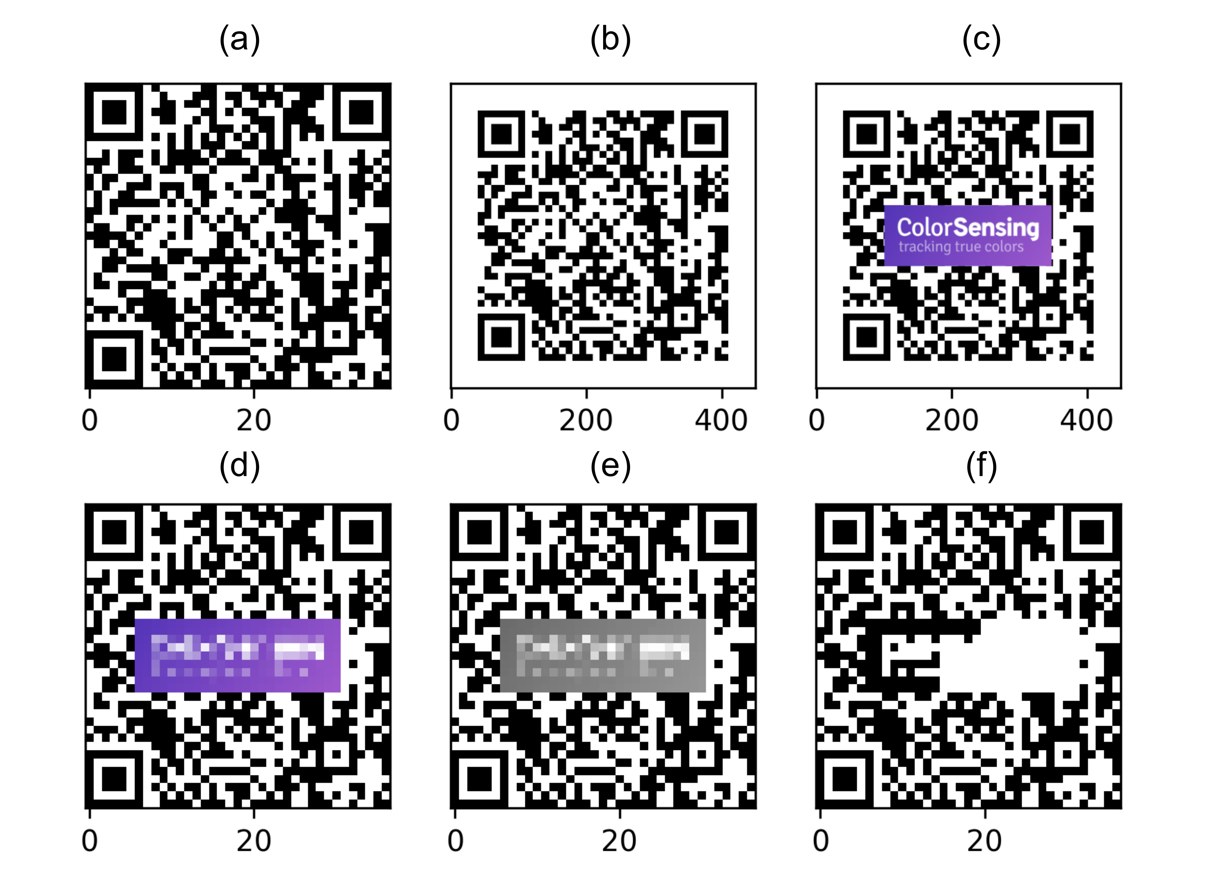
We usually represent signal-to-noise ratio (SNR) from the point of view of signal processing. Thus SNR is the ratio between the ‘signal power’ and the ‘noise power’. Usually, as signals are evaluated over time, this ratio is presented as a root-mean-square average (RMS):
\[\label{eq:snrdef} \mathrm {SNR} ={\frac {P_{\mathrm {RMS, signal} }}{P_{\mathrm {RMS, noise} }}}\]
where \(P_{\mathrm {RMS, signal} }\) and \(P_{\mathrm {RMS, noise} }\) are the average power of the signal and the noise, respectively. Which in turn is equal to:
\[\label{eq:snrdef} \mathrm {SNR} =\left({\frac {A_{\mathrm {RMS, signal} }}{A_{\mathrm {RMS, noise} }}}\right)^{2}\]
where \(A_{\mathrm {RMS, signal} }\) and \(A_{\mathrm {RMS, noise} }\) are the root-mean-square (RMS) amplitude of the signal and the noise. The RMS of a discrete \(x\) variable can be written as:
\[{\displaystyle x_{\text{RMS}}={\sqrt {{\frac {1}{n}}\left(x_{1}^{2}+x_{2}^{2}+\cdots +x_{n}^{2}\right)}}}\]
Then, using this RMS expression and having into account grayscale images can be defined as two-dimensional discrete variables, we can rewrite SNR as follows:
\[\label{eq:snrcalc} \mathrm {SNR} = {\frac {\sum_0^n \sum_0^m (A_{gray}(i, j))^2}{\sum_0^n \sum_0^m (A_{gray}(i, j) - C_{gray}(i, j))^2}}\]
where \(A_{gray} \in [0,1]^{n\times m}\) are the pixels of the QR Code original image ([fig:snrberdefinition].a), which act as a ‘signal image’, \(C_{gray} \in [0,1]^{n\times m}\) are the pixels of the QR Code with the logo in a normalized grayscale ([fig:snrberdefinition].b), the difference between both images acts as the ‘noise image’ ([fig:snrberdefinition].c), and the ratio between their variances is the SNR. Finally, the SNR values can be expressed in decibels using the standard definition:
\[\mathrm {SNR_{dB}} = 10 \ \mathrm {log_{10}}(\mathrm {SNR}).\]
The bit error ratio (BER) is defined as the probability to receive an error when reading a set of bits or, in other words, the mean probability to obtain a \(\mathrm{0}\) when decoding a \(\mathrm{1}\) and to obtain a \(\mathrm{1}\) when decoding a \(\mathrm{0}\):
\[\label{eq:berdef} \mathrm {BER} = \frac{E(N)}{N}\]
where \(N\) is the total amount of bits received, and \(E(N)\) the errors counted in the \(N\) bits. In our case, this translates into the mean probability to obtain a black pixel when decoding a white pixel, or to obtain a white one when decoding a black one. A reformulated BER expression for our binary images is as follows:
\[\label{eq:bercalc} \mathrm {BER} = \frac{\sum_0^n \sum_0^m | A_{bin}(i, j) - C_{bin}(i, j) |}{N}\]
where \(A_{bin} \in \{0,1\}^{n\times m}\) is the binarized version of \(A_{gray} \in [0,1]^{n\times m}\) ([fig:snrberdefinition].d), \(C_{bin} \in \{0,1\}^{n\times m}\) is the binarized version of \(C_{gray} \in [0,1]^{n\times m}\) ([fig:snrberdefinition].e) and \(N = n \cdot m\) are the total pixels in the image. The pixels contributing to the BER are shown in [fig:snrberdefinition].f.
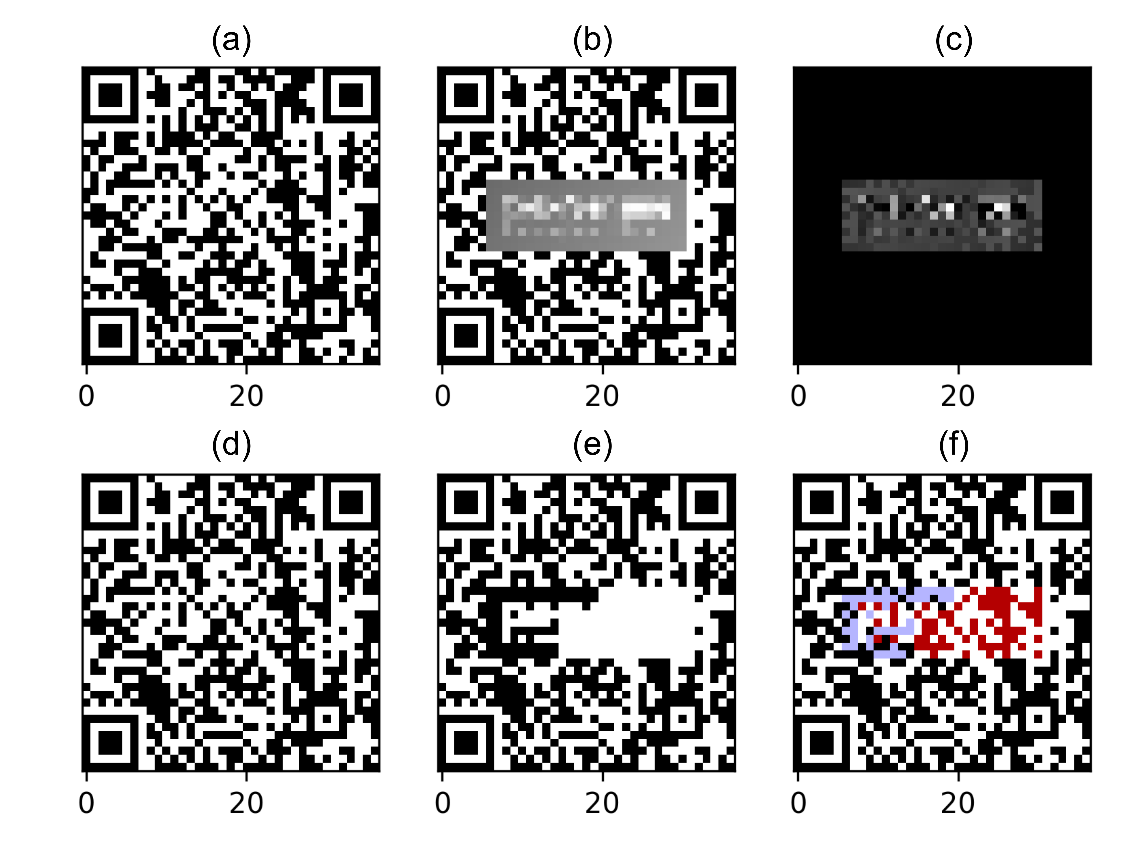
As an example of these calculations, [tab:snrber] shows the results for the computation of the SNR and BER figures for [fig:qrwithlogo] images. As we can see, adding a logo to the pattern represents a noise source that reduces the SNR to 10.53 dB, further noise sources (printing, capture, etc.) will add more noise thus reducing the SNR even more. BER metric shows us the impact of the logo when recovering the digital bits. As we have mentioned before this quantity is directly related to the error correction level needed to encode the QR Code. In this example, with a BER of 8.54%, the poorest error correction level (L, 7%) would not suffice to ensure safe readout of the barcode.
| Measure | Acronym | Value |
|---|---|---|
| Signal-to-Noise ratio | SNR | \(\mathrm{10.53 \ dB}\) |
| Bit error ratio | BER | \(\mathrm{8.54}\) % |
We want to achieve back-compatibility with the QR Code standard. This means that we must still be able to recover the encoded data message from the colored QR Code using a standard readout process (capturing, sampling, desaturating and thresholding).
To make it possible we must place these colors inside the barcode avoiding the protected key areas that ensure its readability. In the rest of the available positions, the substitution of black and white pixels with colors can be regarded as a source of noise added to the digital data pattern. We propose here a method to reduce the total amount of noise and miss-classifications introduced in the QR Code when encoding colors, that is based on the affinity of those colors to black and white (i.e. to which color it resembles the most). To that end, we classify the colors of the palette to be embedded in two groups: pseudo-black and pseudo-white colors.
Initially, let \(G'_{rgb} \in [0,255]^{l \times 3}\) be a set of colors with size \(l\) we want to embed in a QR Code. Then, let us start with the definition of the main steps of our proposal to encode these colors inside a QR Code:
Normalization, the 8-bit color channels (RGB) are mapped to a normalized color representation:
\[\label{eq:normalizationdef} f_{normalize}: [0,255]^{l \times 3} \to [0,1]^{l \times 3}\]
Desaturation, the color channels (RGB) are then mapped into a monochromatic grayscale channel (L):
\[\label{eq:desaturationdef} f_{grayscale}: [0,1]^{l \times 3} \to [0,1]^{l}\]
Binarization, the monochromatic grayscale channel (L) is converted to a monochromatic binary channel (B):
\[\label{eq:binarizationdef} f_{threshold}: [0,1]^{l} \rightarrow \{0,1\}^{l}\]
Colorization, the binary values of the palette colors represent the affinity to black (zero) and white (one) and can be used to create a mapping between the position in the color palette list and the position inside the QR Code matrix (a binary image). This mapping will also depend on the geometry of the QR Code matrix (where are the black and the white pixels placed) and an additional matrix that protects the key zones of the QR Code (a mask that defines the key zones):
\[\label{eq:mappingdef} f_{mapping} : \{0,1\}^{l} \times \{0,1\}^{n\times m} \times \{0, 1\}^{n \times m} \to \{0, \dotsc, l+1\}^{n \times m}\]
Once the mapping is computed, a function is defined to finally colorize the QR Code, which renders an RGB image of the QR Code with embedded colors:
\[\label{eq:colorizationdef} f_{colorize} : \{0,1\}^{n\times m} \times [0,1]^{l \times 3} \times \{0, \dotsc, l+1\}^{n \times m} \to [0,1]^{n\times m \times 3}\]
Subsequently, to create the pseudo-black and pseudo-white colors subsets, we must define the implementation of these functions. These definitions are arbitrary, i.e. it is possible to compute a grayscale version of a color image in different ways. Our proposed implementation is intended to resemble the QR Code readout process:
Normalization, \(f_{normalize}\) will be a function that transforms a 24-bit color image (RGB) to a normalized color representation. We used a linear rescaling factor for this:
\[\label{eq:normalizationimpl} G_{rgb} (k, c) = f_{normalize} (G'_{rgb}) = \frac{1}{255} G'_{rgb} (k, c)\]
where \(G'_{rgb} \in [0,255]^{l \times 3}\) is a list of colors with a 24-bit RGB color depth and \(G_{rgb} \in [0,1]^{l \times 3}\) is the normalized RGB version of these colors.
Desaturation, \(f_{grayscale}\) will be a function that transforms the color channels (RGB) to a monochromatic grayscale channel. We used an arithmetic average of the RGB pixel channels:
\[\label{eq:desaturationimpl} G_{gray}(k) = f_{grayscale}(G_{rgb}) = \frac{1}{3} \sum_{c=0}^3 G_{rgb}(k,c)\]
where \(G_{rgb} \in [0,1]^{l \times 3}\) is the normalized RGB color palette and \(G_{gray} \in [0,1]^{l}\) is the grayscale version of this color palette.
Binarization, \(f_{threshold}\) will be a function that converts the monochromatic grayscale channel (L) to a binary channel (B). We used a simple threshold function with a thresholding value of \(\mathrm{0.5}\):
\[\label{eq:binarizationimpl} G_{bin} (k) = f_{threshold}(G_{gray}) = \begin{cases} 0 & G_{gray}(k) \leq 0.5 \\ 1 & G_{gray}(k) > 0.5 \\ \end{cases}\]
where \(G_{gray} \in [0,1]^{l}\) is the grayscale version of the color palette and \(G_{bin} \in \{0,1\}^{l}\) is its binary version, which describes the affinity to black (\(\mathrm{0}\)) and white (\(\mathrm{1}\)) colors.
Colorization, \(f_{color}\) will be a function that will render a RGB image from the QR Code binary image and the palette colors by using a certain mapping. We used this function to implement it:
\[\label{eq:colorizationimpl} \begin{split} C_{rgb} (i, j,k) = f_{color} (A_{bin}, G_{rgb}, M) = \begin{cases} A_{bin}(i,j) & M(i,j) = 0 \\ G_{rgb}(p-1,k) & M(i,j) = p > 0 \\ \end{cases} \end{split}\]
where \(A_{bin} \in \{0,1\}^{n\times m}\) is the original QR Code binary image, \(G_{rgb} \in [0,1]^{l \times 3}\) is a color palette to be embedded in the image, \(C_{rgb} \in [0,1]^{n\times m \times 3}\) is the colorized QR Code image, and \(M \in \{0, \dotsc, t\}^{n \times m}\) is an array mapping containing the destination of each one of the colors of the palette into the 2D positions within the image. We propose to use \(G_{bin}\) ([eq:binarizationimpl]) to create \(M\). This mapping will also depend on the geometry of the QR Code image (where are the black and the white pixels placed) and an additional matrix that protects the key zones of the QR Code (a mask which defines the key zones), this mapping will be \(f_{mapping}\), it has the general form:
\[\label{eq:mappingimpl} M = f_{mapping} (G_{bin}, A_{bin}, Z)\]
where \(M \in \{0, \dotsc, t\}^{n \times m}\) is the array mapping, \(G_{bin} \in \{0,1\}^{l}\) is the affinity to black or white of each color in the palette, \(A_{bin} \in \{0,1\}^{n\times m}\) is the original QR Code binary image and \(Z \in \{ 0, 1 \}^{n \times m}\) is a mask that protects the QR Code key patterns to be overwritten by the palette. One possible implementation of \(f_{mapping}\) ([eq:mappingimpl]) is shown in [algorithm], where the colors of the palette are mapped to positions of the QR Code based on their affinity to black and white. For each one of these two classes, the particular assignment of a color to one of the many possible pixels of the class (either black or white) is fully arbitrary and allows for further design decisions. In this implementation of the mapping, we choose to assign the colors in random positions within the class. In other applications, interested e.g. in preserving a certain color order, additional mapping criteria can be used as shown below. Anyhow, preserving the assignment to the black or white classes based on the color affinity is key for back-compatibility.
\(W_{color} \leftarrow[]\)
\(B_{color} \leftarrow[]\)
\(p \leftarrow
lenght(W_{color})\)
\(q \leftarrow
lenght(B_{color})\)
\(W_{pos} \leftarrow[]\)
\(B_{pos} \leftarrow[]\)
\(W'_{pos} \leftarrow\) Select
\(p\) random values of \(W_{pos}\)
\(B'_{pos} \leftarrow\) Select
\(q\) random values of \(B_{pos}\)
\(M \leftarrow\{0\}_{i, j}\ \ \forall i \in
\{0, \dotsc, n\}\) and \(j \in \{0,
\dotsc, m\}\)
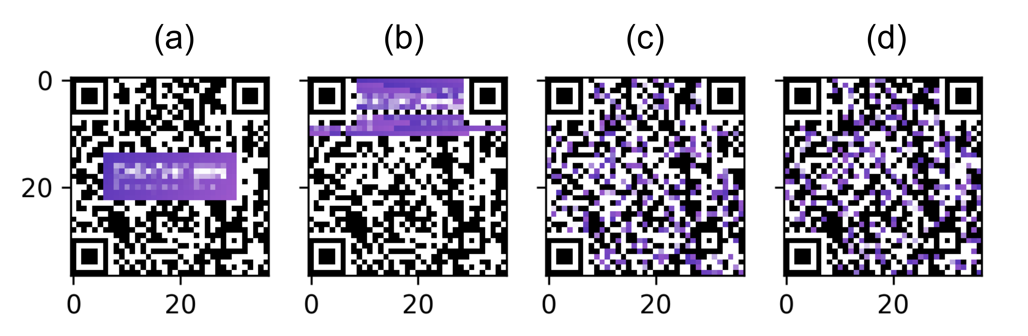
Moreover, to illustrate how different placement mappings affect the readout process, we will consider 4 different situations, where \(f_{mapping}\) plays different roles, and we will compute their SNR and BER metrics:
Logo. When a logo-like pattern is encoded, \(G_{rgb}\) will be the colors of the logo and \(M_{logo}\) will be a mapping that preserves the logo image, overlaid on top of the original QR Code image ([fig:snrbercomparisson].a.).
Sorted. We are going to use the colors of the logo (thus \(G_{rgb}\) will be the same as before), but we are going to place them on top of the QR Code, sorting them as they appear in the color list. \(M_{sorted}\) will establish that the first color goes to the first available position inside \(A_{gray}\) pixels, etc. ([fig:snrbercomparisson].b.).
Random. Again we use the same colors of the logo (\(G_{rgb}\) remains the same) but now \(M_{random}\) defines a random mapping of the palette into the available positions of \(A_{gray}\) ([fig:snrbercomparisson].c.).
Grayscale. Our proposed method. Same as before, but the now random assignment of \(M_{gray}\) respects the rule that pseudo-white colors are only assigned to white pixels of \(A_{gray}\), and pseudo-black only to the black ones, as described in [algorithm] ([fig:snrbercomparisson].d.).
| Measure | Logo | Sorted | Random | Grayscale |
|---|---|---|---|---|
| SNR | \(\mathrm{10.53 \ dB}\) | \(\mathrm{10.27 \ dB}\) | \(\mathrm{10.35 \ dB}\) | \(\mathrm{12.23 \ dB}\) |
| BER | \(\mathrm{8.55}\) % | \(\mathrm{8.33}\) % | \(\mathrm{8.62}\) % | \(\mathrm{0.00}\) % |
Finally, [tab:snrberlogocolors] shows the SNR and BER figures for the four mappings (exemplified in the images of [fig:snrbercomparisson]). Using the grayscale approach to encode colors by their resemblance to black and white colors leads to much lower noise levels. Since the original data of the QR Code can be seen as a random distribution of white and black pixels, \(M_{sorted}\) and \(M_{random}\) mappings yield similar results to \(M_{logo}\), encoding the logo itself. Meanwhile, \(M_{gray}\) mapping shows us a \(\mathrm{0}\)% BER, and an almost \(\mathrm{2dB}\) SNR increase. This suggests that our proposal can be an effective way to embed colors into QR Code in a back-compatible manner (see [fig:colorqrflow]), as it is demonstrated in the following sections.
Experiments were designed to test our proposed method, we carried out 3 different experiments where QR Codes were filled with colors and then transmitted through different channels. In all experiments, we calculated the SNR and BER as a measure of the signal quality of each QR Code once transmitted through different channels. Also, we checked the direct readability by using a QR Code scanner before and after going through the channels. [tab:experiments] contains a summary of each experiment designed. A detailed explanation of the experimental variables is provided below.
| All experiments | Values | Size |
|---|---|---|
| Color substitution (%) | 1, 5, 10, 15, 20, 30, 40, 50, 60, 70, 80, 100 | 12 |
| Colorized zone | EC, D, EC&D | 3 |
| Colorizing method | Random, Grayscale | 2 |
| Experiment 1 | Values | Size |
| Digital IDs | from 000 to 999 | 1000 |
| QR version | 5, 6, 7, 8, 9 | 5 |
| Channels | Empty, Image augmentation | 1 + 1 |
| Experiment 2 | Values | Size |
| Digital IDs | 000 | 1 |
| QR version | 5, 6, 7, 8, 9 | 5 |
| Channels | Empty, | |
| Image augmentation | 1 + 1000 | |
| Experiment 3 | Values | Size |
| Digital IDs | 000 | 1 |
| QR version | 5 | 1 |
| Channels | Empty, Colorimetry setup | 1 + 25 |
We choose our random color palette \(G_{rgb}\) for the experiments to be representative of the RGB space. Nevertheless, \(G_{rgb}\) should be random in a way that it is uniformly random in the grayscale space L. But if we define three uniform random RGB channels as our generator, we will fail to accomplish a grayscale uniform random channel. This is due to the fact that when computing the L space as a mean of the RGB channels, we are creating a so-called Irwin-Hall uniform sum distribution [134] (see [fig:colorgenarots].b.). In order to avoid this, we propose to first generate the L channel as a uniform random variable, then generate RGB channels which will produce these generated L channel values (see [fig:colorgenarots].b.).
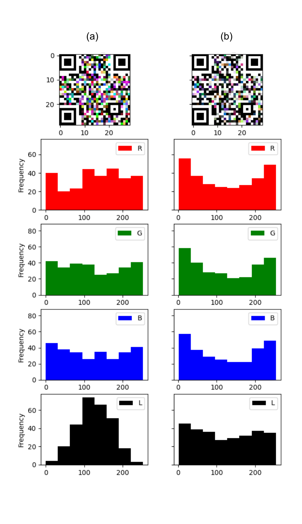
During the different experiments, we will be filling QR Codes with a palette of random colors \(G_{rgb}\). The color substitution factor ranged from only 1% of the available pixel positions in a QR Code replaced with colors up to 100% (see [fig:colorplacement]). Evidently, each QR Code version offers different numbers of pixels and thus positions available for color substitution.
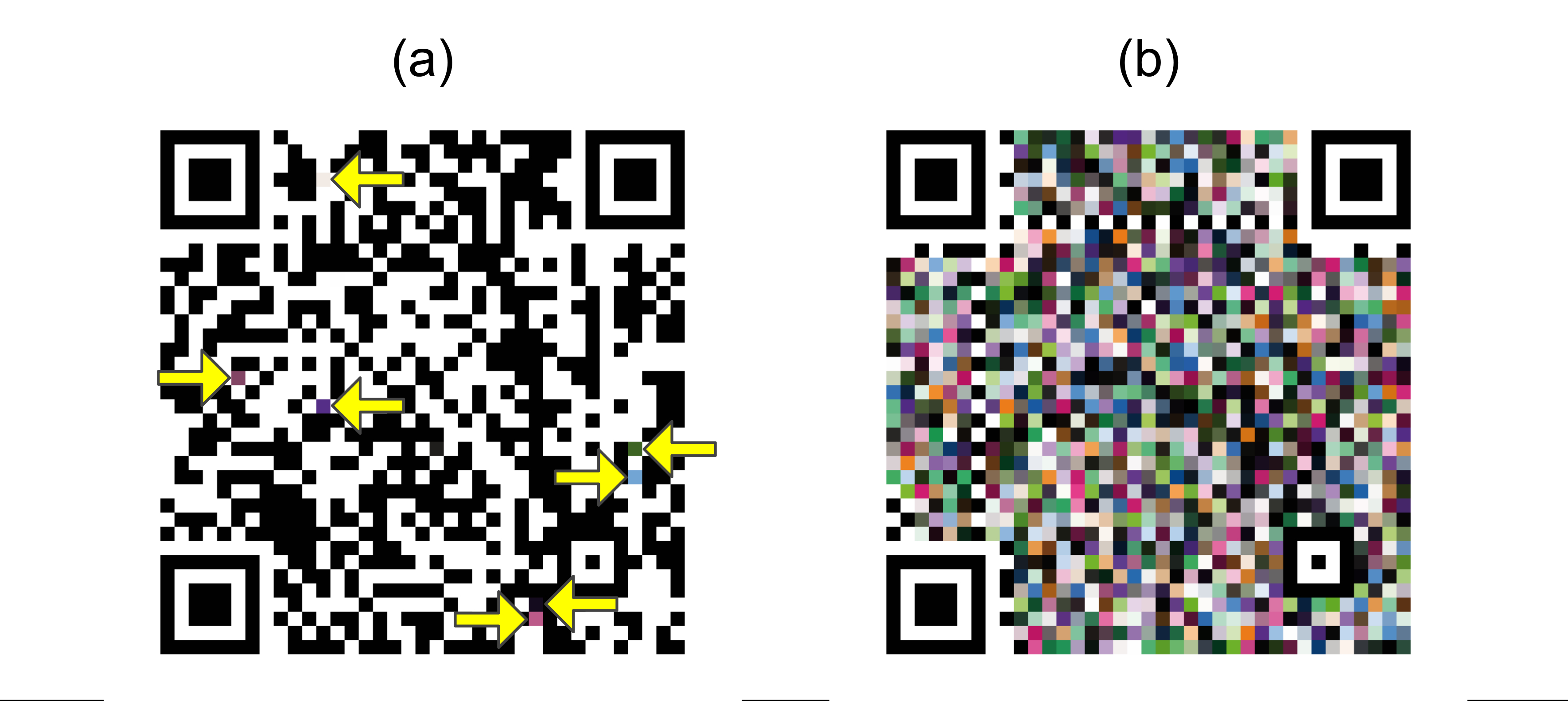
Our back-compatibility proposal starts avoiding the substitution of colors in key protected areas of the QR Code. This can be implemented with a \(Z\) mask (see [algorithm]). In our experiments, we used 3 masks (see [fig:coloredareas]):
\(Z_{EC\&D}\), that excludes only the key protected areas and allows covering with colors all the error correction and data regions (see details in [ch:3]),
\(Z_{EC}\), that only allows embedding colors in the error correction,
\(Z_D\), with colors only in the data.
Once we have restricted ourselves to these \(Z\) masks, we will embed the colors following a \(M\) mapping. We propose to use \(M_{random}\) and \(M_{gray}\) presented before (see [fig:snrbercomparisson].c. and [fig:snrbercomparisson].d.).
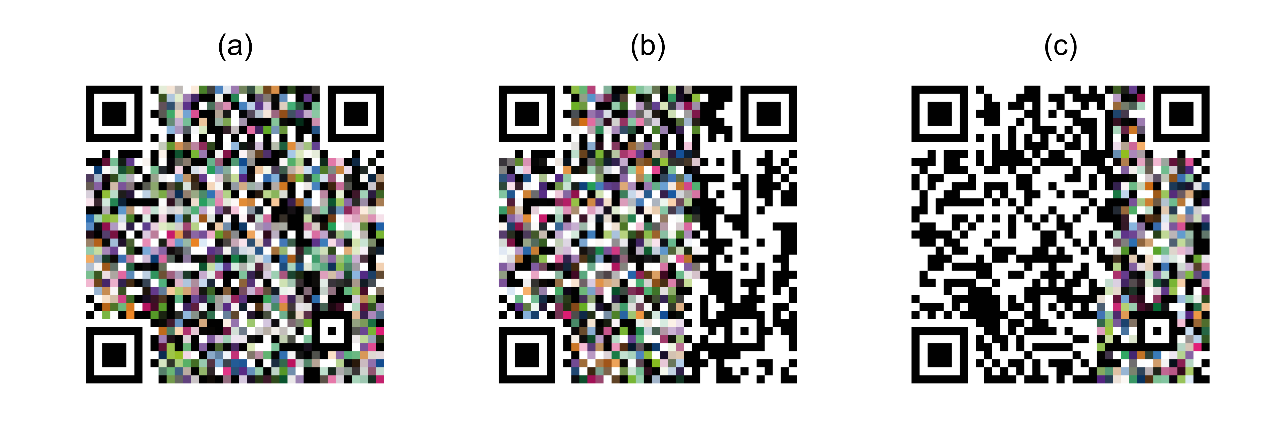
The encoded data and the version of the QR Code will shape the actual
geometry of the barcode, thus it will determine the \(A_{gray}\) pixels. To generate the
barcodes, we choose as payload data a URL with a unique identifier such
as https://color-sensing.com/#000, where the numbers after
‘#’ range from 000 to 999 to make
the barcodes different from each other. Also, the QR Code selected
versions ranged from 5 to 9, to test and exemplify the most relevant
computer vision pattern variations defined in the QR Code standard. For
all of these barcodes, we used the highest level of error correction of
QR Code standard: the H level, which provides a 30% of error
correction.
The use of QR Codes in real world conditions imply additional sources of error, like differences in printing, different placements, ambient light effects, effects of the camera and data processing, etc. All these factors can be regarded as sources of noise in a transmission channel.
We considered 3 different channels for the experiments:
Empty. A channel where there is no color alteration due to the channel. It was used as a reference, to measure the noise level induced by the colorization process (see [fig:channels].a).
Image augmentation. With a data augmentation library [121] we generated images that mimic different printing processes and exposure to different light conditions. With this tool we also applied Gaussian blur distortions, crosstalk interferences between the RGB channels and changed contrast conditions. (see [fig:channels].b).
Physical printouts exposed to controlled illumination. We actually printed the QR Codes and captured them with a fixed camera (Raspberry Pi 3 with a Raspberry Pi Camera v2) [135] under different illumination-controlled conditions (Phillips Hue Light strip) [136]. The camera was configured to take consistent images. The light strip was configured to change its illumination conditions with two subsets of lights: white light (9 color temperatures from 2500K to 6500K) and colored light (15 different colors sampling evenly the CIExyY space) (see [fig:channels].c).
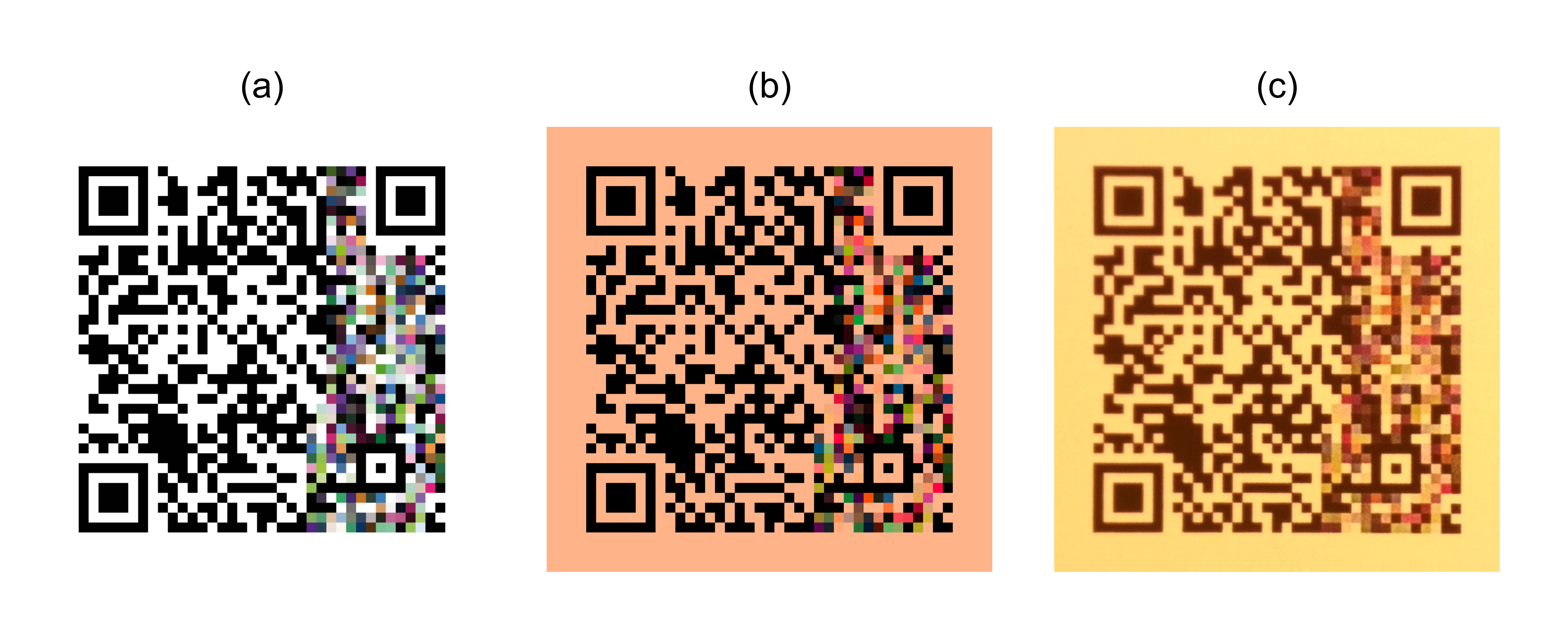
Let us start with the results of Experiment 1, where 360.000 different color QR Codes were encoded (see [tab:experiments]). Then, the SNR and BER were computed against an empty channel (only the color placement was taken into account as a source of noise). Results show only data from those QR Codes where colors were placed using the \(Z_{EC\&D}\) mask (see details in [subsec:qrcodeversionsandids]), reducing our dataset to 120.000 QR Codes. [fig:snrberemptychannel] shows aggregated results of the SNR and BER as a function of the color substitution ratio, for \(M_{random}\) and \(M_{gray}\) mappings data is averaged for all QR Code versions (5, 6, 7, 8 and 9) and for all 1000 different digital IDs. These results indicate that the SNR and BER are independent of the QR Code versions and the QR Code digital data, since the standard deviations of these figures (shadow area in [fig:snrberemptychannel]) that average different versions and digital IDs are very small. Only the BER for \(M_{random}\) shows a narrow deviation. Of course, all these deviations increased when noise was added (see further results).
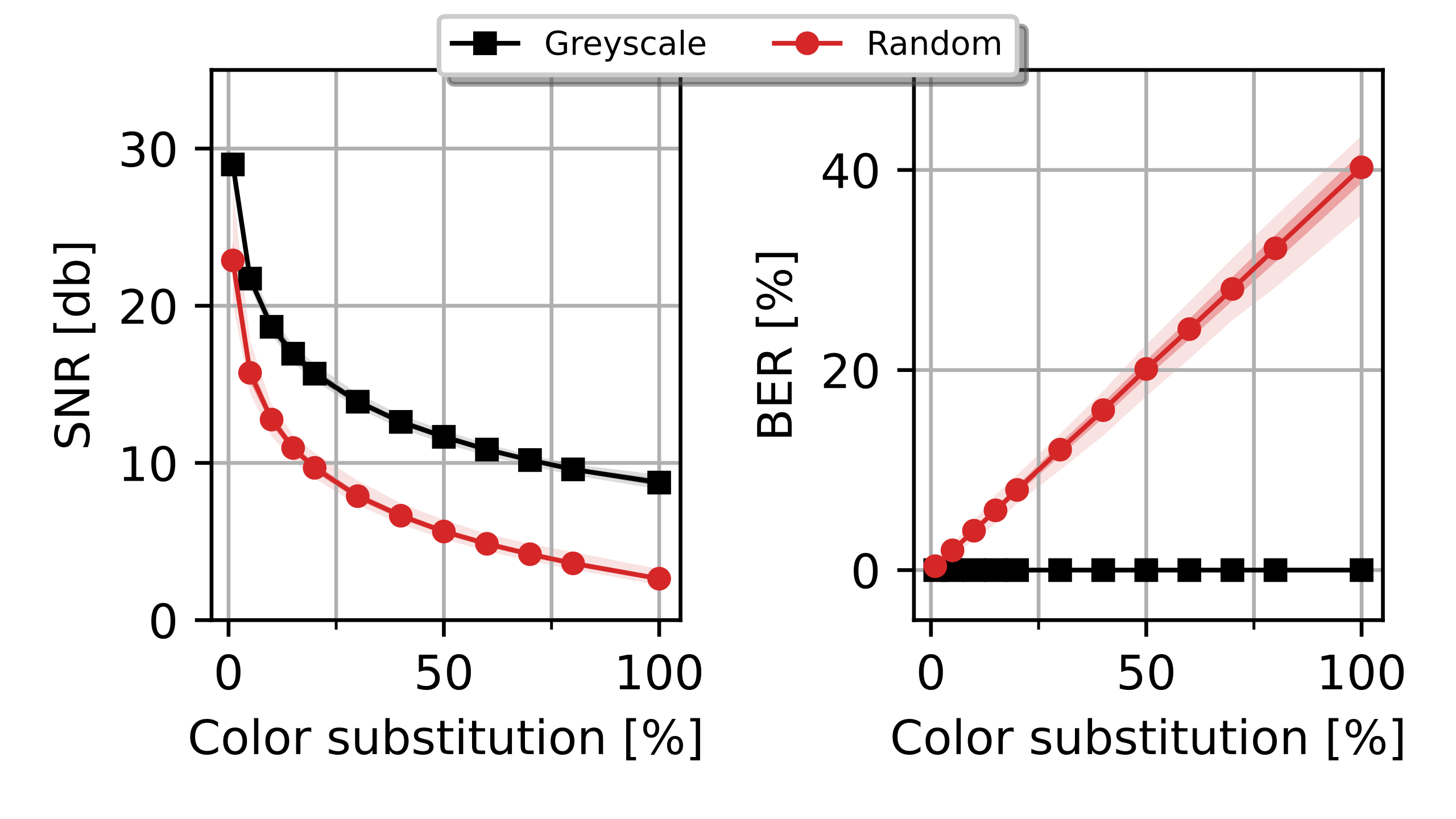
Regarding the SNR, it decreases for both \(M_{random}\) and \(M_{gray}\) when the total amount of colors increases. We found that our \(M_{gray}\) proposal (affinity towards black and white) is 6 dB better than \(M_{random}\), regardless of the quantity of colors embedded, the data, or the version of the QR Code. This means that our proposal to place colors based on their grayscale value is 4 times less noisy than a random method.
Concerning the BER, results show that, before including the effects of a real noisy channel, our placement method leads to a perfect BER score (\(\mathrm{0}\)%). Instead, with a random substitution, and even in an ideal channel, BER increases linearly and reaches up to a \(\mathrm{40\%}\) of BER. Taking into account the QR Code resemblance to a pseudo-random pattern, the maximum BER in this scenario is \(\mathrm{50\%}\). This slightly better result can be attributed to the fact that we are not tampering with the key protected patterns of the QR Code (finder, alignment, …).
Results from Experiment 1 showed that the SNR and BER results are independent from the data encoded in the QR Code. Based on this finding, we reduced the amount of different IDs encoded to only one per QR Code version and increased the number of image augmentation channels to 1000. This was the key idea of Experiment 2, and by doing this we achieved the same statistics of a total 360.000 results, from 3.600 QR Codes sent though 1.000 different channels. Focusing again only on the QR Codes that are color embedded using the whole zone (\(Z_{EC\&D}\)) we ended up with 120.000 results to calculate the corresponding SNR and BER (see [fig:snrberaugmentationchannel]).
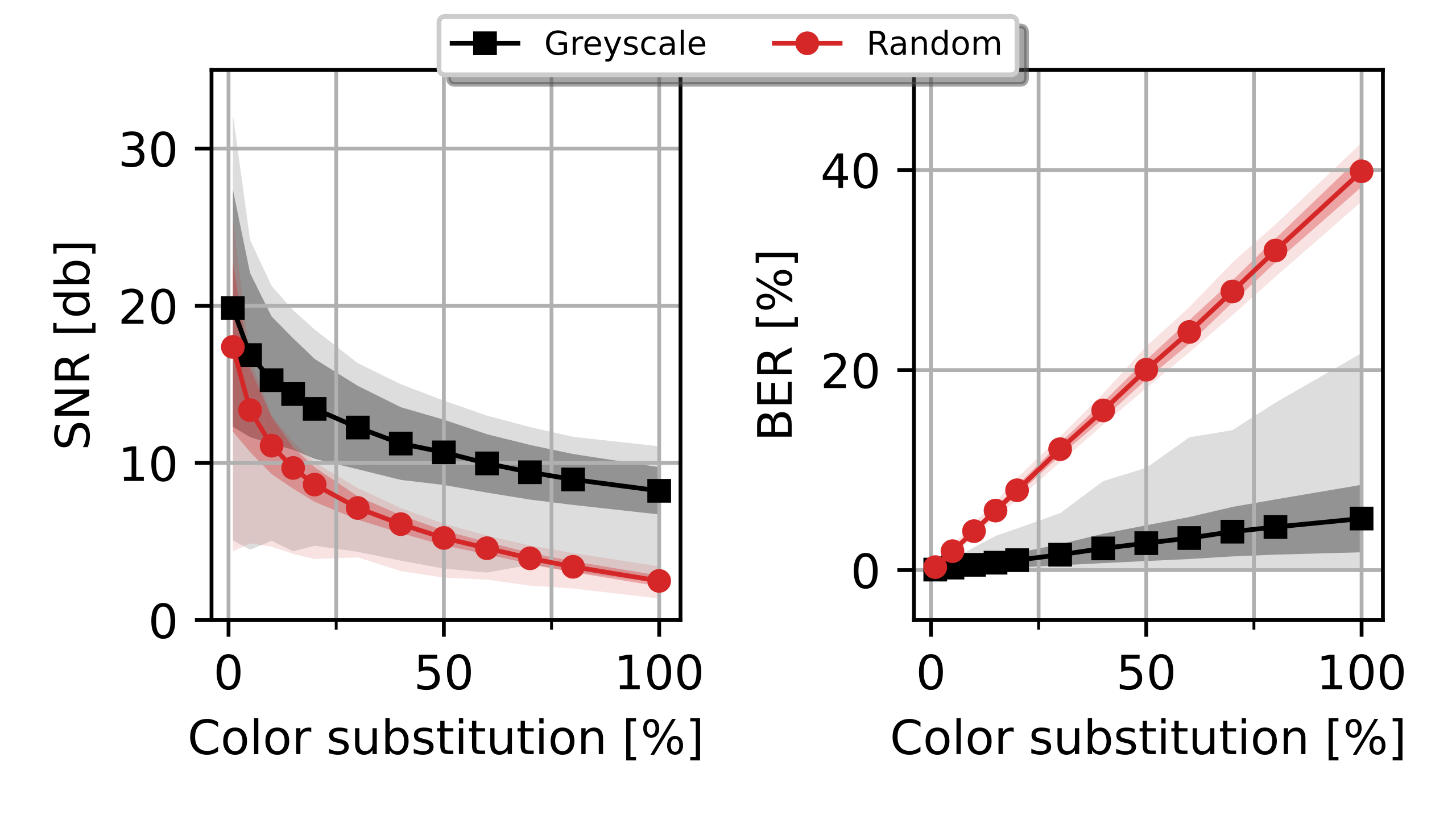
Regarding the SNR, it worsened in comparison with Experiment 1, because now the image augmentation channel is adding noise (see details in [subsec:channels]). The 6 dB difference between \(M_{random}\) and \(M_{gray}\) remains for higher color substitution. This can be explained because the noise generated by the color placement is larger than the noise generated by the channel when increasing the amount of colors.
Concerning the BER, it increased up to an average value of about 7% for \(M_{gray}\) method due to the influence of a noisy channel. In the most extreme cases (channel with the lowest SNR and for the maximum color substitution ratio), BER values do not exceed 20%. Instead, the augmentation channel does not seem to increase the BER for \(M_{random}\); essentially because it is already close to the theoretical maximum.
We have also observed (see [fig:snraugmentationchannelversions]) that the impact of the channel noise on the SNR and BER figures of \(M_{random}\) and \(M_{gray}\) are mostly independent of the QR Code version. Therefore, we can expect that the level of resilience to noise offered by one or another mapping will remain, independently of the data to encode or the QR Code version needed. That is the reason why we removed the QR Code version from the set of variables to explore in the Experiment 3.
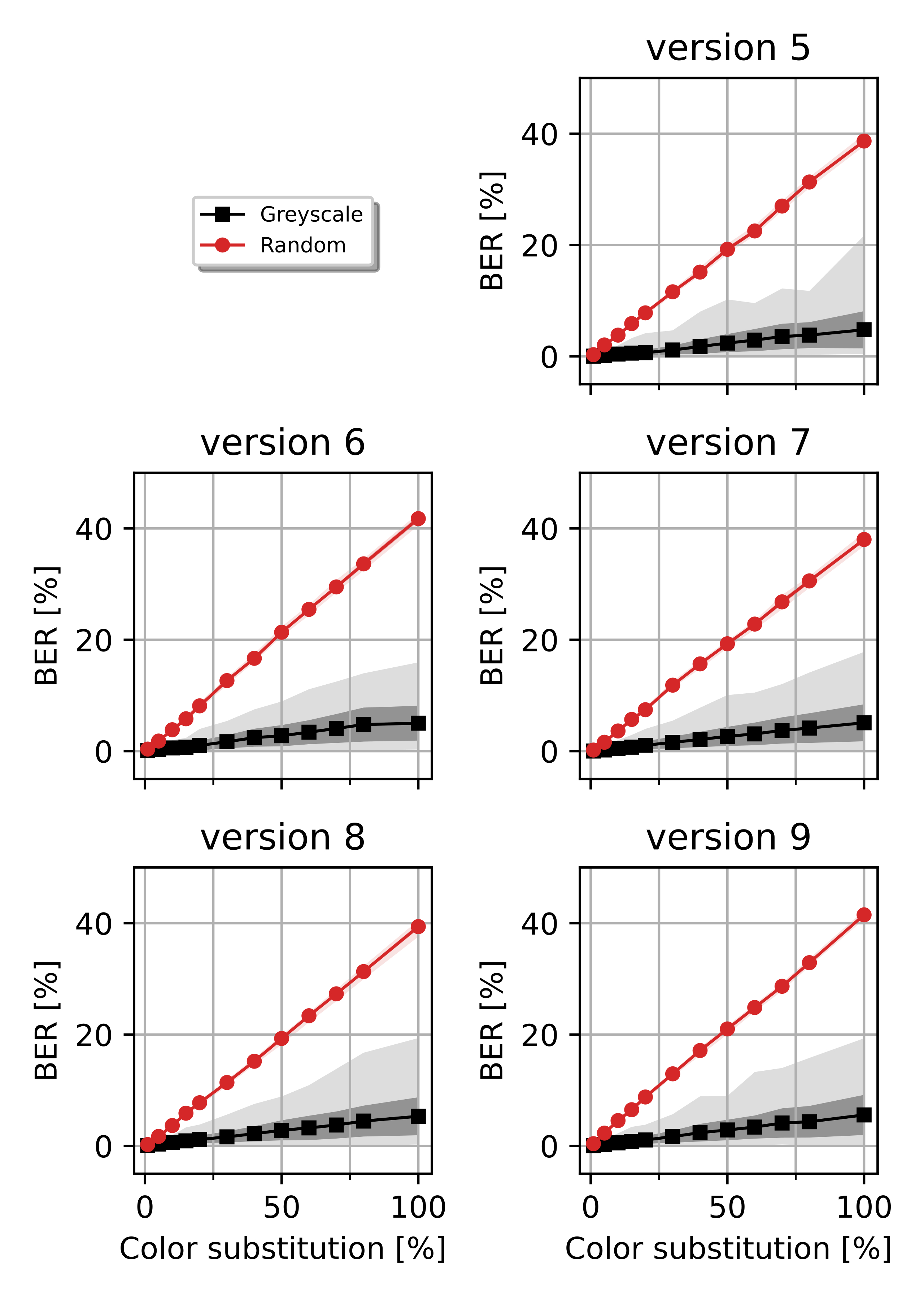
Experiment 3 consisted of only one QR Code v5 (1 ID, 1 version) being colored in 72 different ways (12 color insertion ratios, 2 color placement mappings –\(M_{random}\) and \(M_{gray}\)– and 3 different zones to embed colors –\(Z_{EC\&D}\), \(Z_{EC}\) and \(Z_{D}\)–), then printed and exposed to a colorimetry setup with a total of 25 different color illumination conditions captured with a digital camera. We performed this experiment as a way to check if the proposed method and the results obtained with the image augmentation channel held in more extreme, and real, capturing conditions. This experiment led to a dataset of 1.800 images acquired from the real world. The calculations of the SNR and the BER were based on those images with colors placed with the \(Z_{EC\&D}\) mask, reducing our dataset to 600 results (see [fig:snrberrealchannel]).
Regarding the SNR, as our real channel was quite noisy, averaged values sank more than 10 dB, for all the color substitution ratio and for \(M_{random}\) and \(M_{gray}\). Here, the huge advantage of 6dB observed before for \(M_{gray}\) was not so evident, since the channel was now the main source of noise. This should serve to illustrate that our proposed method starts with an initial advantage in ideal conditions with respect to the random mapping method, which can diminish due to the channel noise but will always perform better.
Regarding the BER, for \(M_{gray}\), the BER values did not increase relative to the image augmentation channel, both distributions overlap in the range of 7-10% of BER. For \(M_{random}\), the linear maximum behaviour up to a BER of 40% is also shown in this situation. As shown in further sections, although noise levels from both methods are similar in practical applications, the difference in how they are translated into BER determines the better performance of the grayscale mapping.
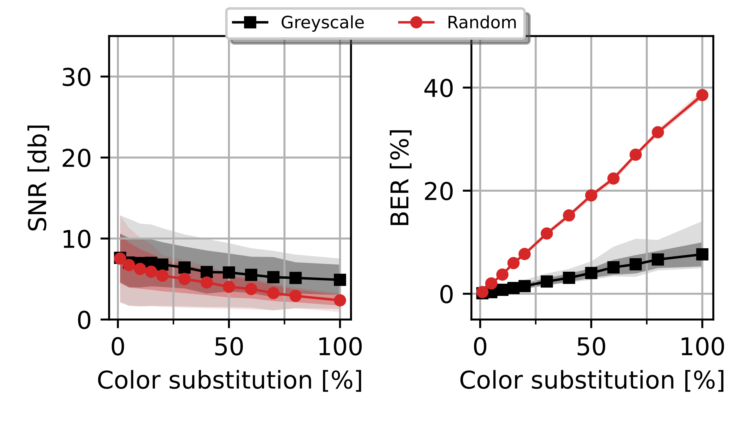
Up to this point, results show how embedding colors in the QR Codes might increase the probability of encountering bit errors when decoding those QR Codes. Results also indicate that our back-compatible method can reduce the average probability of encountering a bit error from \(\mathrm{40\%}\) to \(\mathrm{7-10\%}\), enabling proper back-compatible QR Code scan using the error correction levels included in the standard that can tolerate this amount of error (levels Q and H). This is a necessary but not sufficient demonstration of back-compatibility.
We must also be sure that the new method offers QR Codes fully readable with conventional decoders. To assess this readability, we checked the integrity of the data of all the QRs in our experiments using ZBar, a well-established barcode scanner widely used in the literature [56], [122]. We calculated the success ratio at each color substitution ratio as the amount of successfully decoded QR Codes by ZBar divided by the total amount of QR Codes processed. Also, we analyzed separately the results obtained when embedding colors in the 3 different zones (\(Z_{EC\&D}\), \(Z_{EC}\) and \(Z_D\) masks), in order to identify further relevant behaviours.
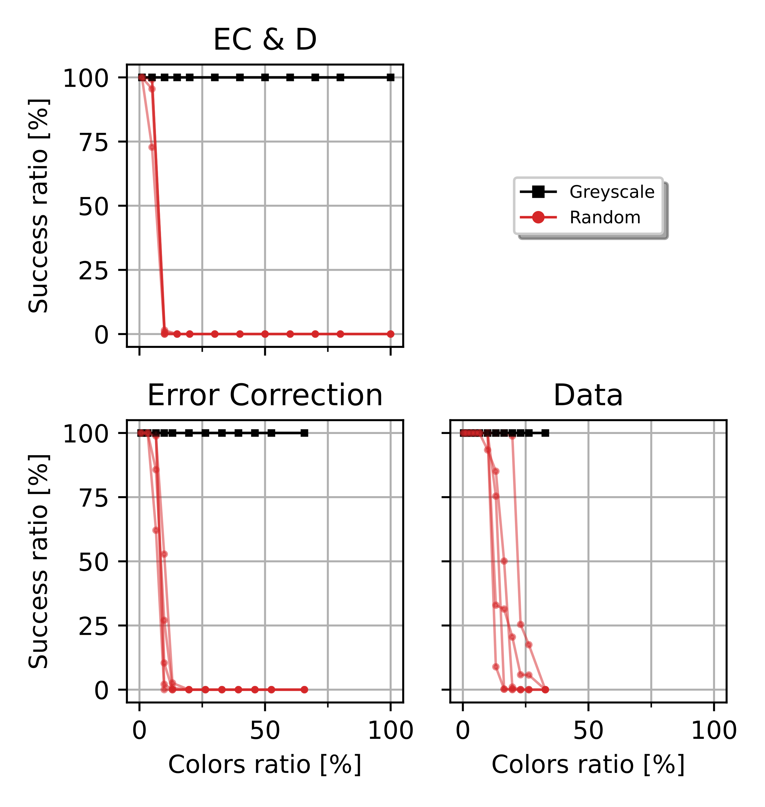
On the one hand, readability results of the QR Codes of Experiment 1 (channel without noise) are shown in [fig:successratioemptychannel]. \(M_{gray}\) (the proposed method) scores a perfect readability, no matter the insertion zone. This is because \(M_{gray}\) does not actually add BER when colors are inserted. Instead, \(M_{random}\) (the random method) is extremely sensitive to color insertion, and the readability success rate decays rapidly as the number of inserted colors increases. As seen in Experiment 1, the Data zone (\(Z_D\)) seems the most promising to embed the largest fraction of colors.
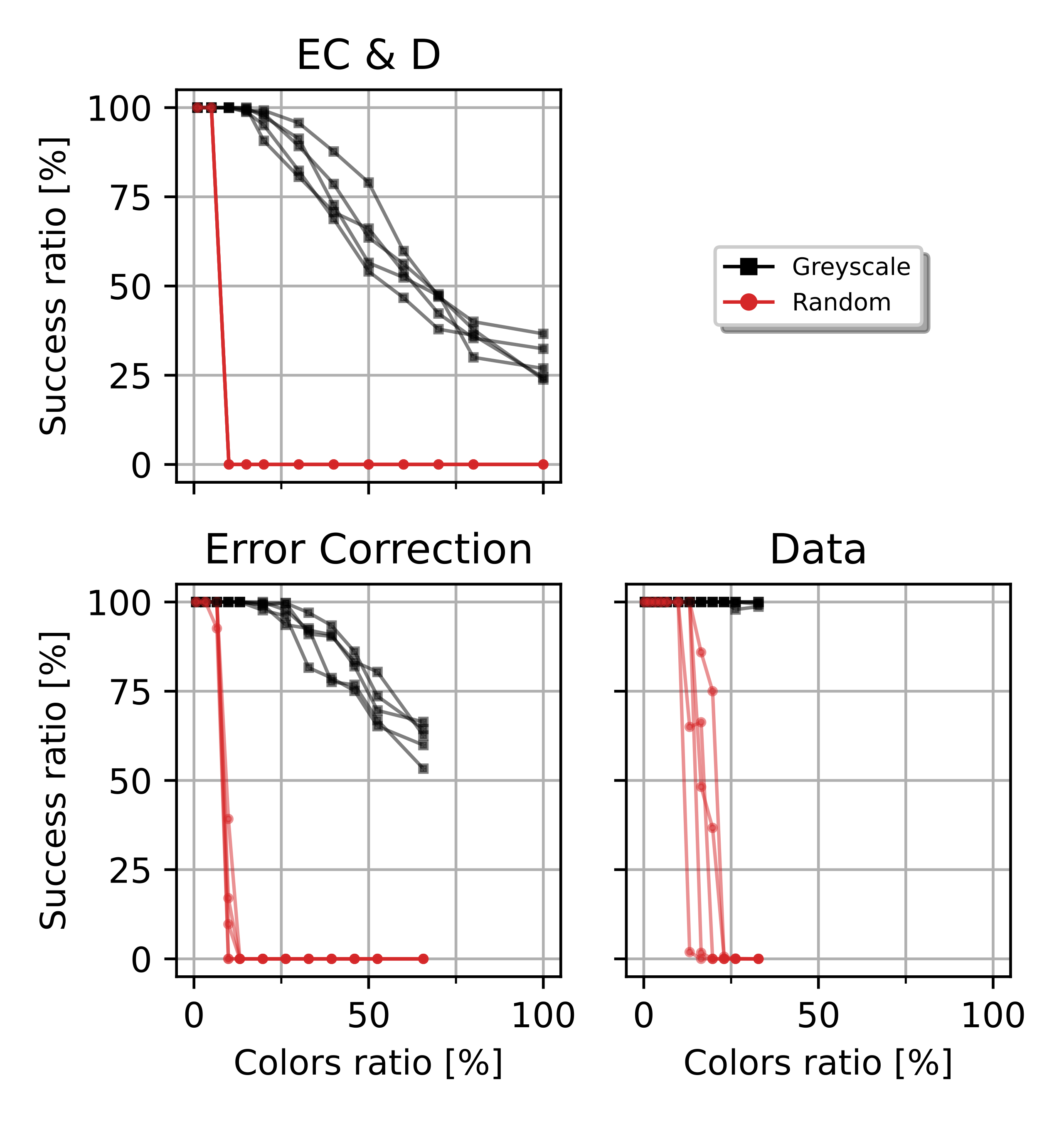
On the other hand, results after passing through the noisy channels of Experiment 2 and Experiment 3 are shown in [fig:successratioaugmentationchannel] and [fig:successratiorealchannel], respectively. Clearly, the noise of the channel also affects the readability of \(M_{gray}\) mapping, but the codes built this way are much more resilient and can allocate a much larger fraction of colors without failing. Even more: if colors are only placed in the Data (\(Z_D\)) encoding zone, grayscale mapped color QR Codes remain fully readable until all the available pixels of the zone are occupied.
To get a practical outcome of these results, one should translate the color substitution ratios into the actual amount of colors that these ratios mean when using different encoding zones in QR Codes with different versions. [tab:results] summarizes these numbers grouped by encoding zone, the QR Code version. Results compare the maximum number of colors that can be allocated using each one of the mapping methods (grayscale vs. random) with at least a \(\mathrm{95}\)% of readability. Experience shows that beyond this \(\mathrm{5}\)% of failure, the user experience is severely damaged.
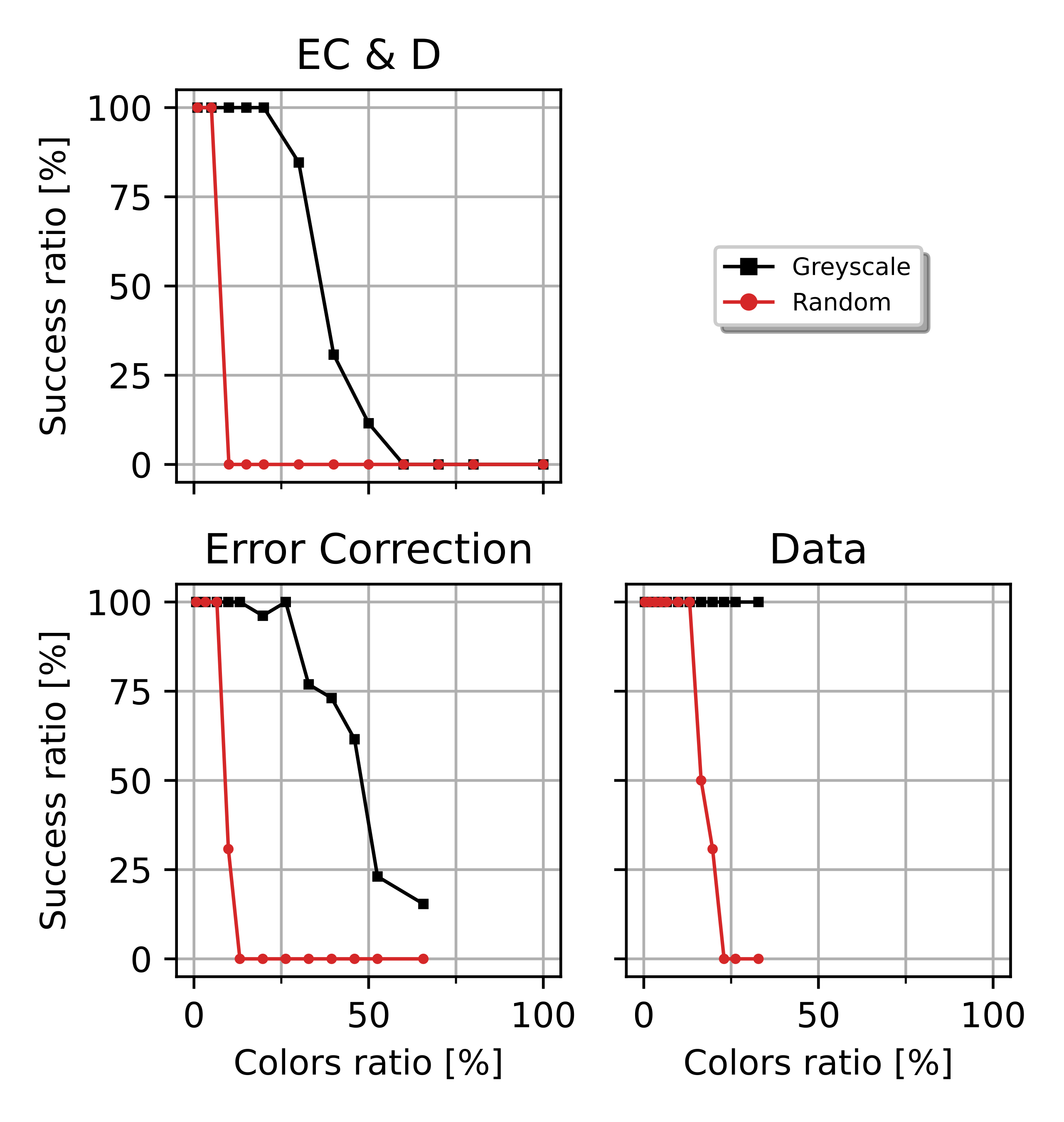
Clearly, the \(M_{gray}\) mapping allows for allocating between \(\mathrm{2x}\) to \(\mathrm{4x}\) times more colors than a naive \(M_{random}\) approach. Interestingly, restricting the placement of colors to the data zone (\(Z_D\)) leads to a much larger number of colors, in spite of having less pixels available; being the error correction (\(Z_{EC}\)) the less convenient to tamper with. In the best possible combination (\(M_{gray}\) mapping, \(Z_D\) zone, \(\mathrm{v9}\) –the largest version studied–) our proposal reaches an unprecedented number of colors that could be embedded close to 800. As a matter of fact, this could mean sampling a 3-dimensional color space of 24 bits resolution (i.e. sRGB) with \(9^3\) colors evenly distributed along each axis.
Needless to say, that such figures can be systematically increased with QR Codes of higher versions. To get a specific answer to the question of how many colors can be be embedded as a function of the QR Code version in the best possible conditions -data zone (\(Z_D\)) with our grayscale mapping (\(M_{gray}\))-, we generated a specific dataset of QR Codes with versions running from \(\mathrm{v3}\) to \(\mathrm{v40}\), and checked their \(\mathrm{95}\)% readability in the conditions of Experiment 2 through 50 image augmentation channels (see [fig:datacapacity]). Results indicate that thousands of colors are easily to reach, with a theoretical maximum of almost \(\mathrm{10000}\) colors with QR Codes \(\mathrm{v40}\). In real life, however, making these high version QR Codes readable with conventional cameras at reasonable distances means occupying quite a lot of space (about \(\mathrm{5}\) inches for a QR Code \(\mathrm{v40}\)). That size, though, is comparable to that of a ColorChecker pattern but giving access to thousands of colors instead of only tens.
r|r@r|r@r|r@r & & &
& & & & & &
& 322 & 54 &
282 & 70 &
352 & 141
6 & 206 & 69
& 448 & 90 &
464 & 139
7 & 314 & 78
& 520 & 104
& 512 &
205
8 & 387 & 97
& 499 & 125
& 672 &
269
9 & 467 & 117
& 461 & 77 &
784 & 235
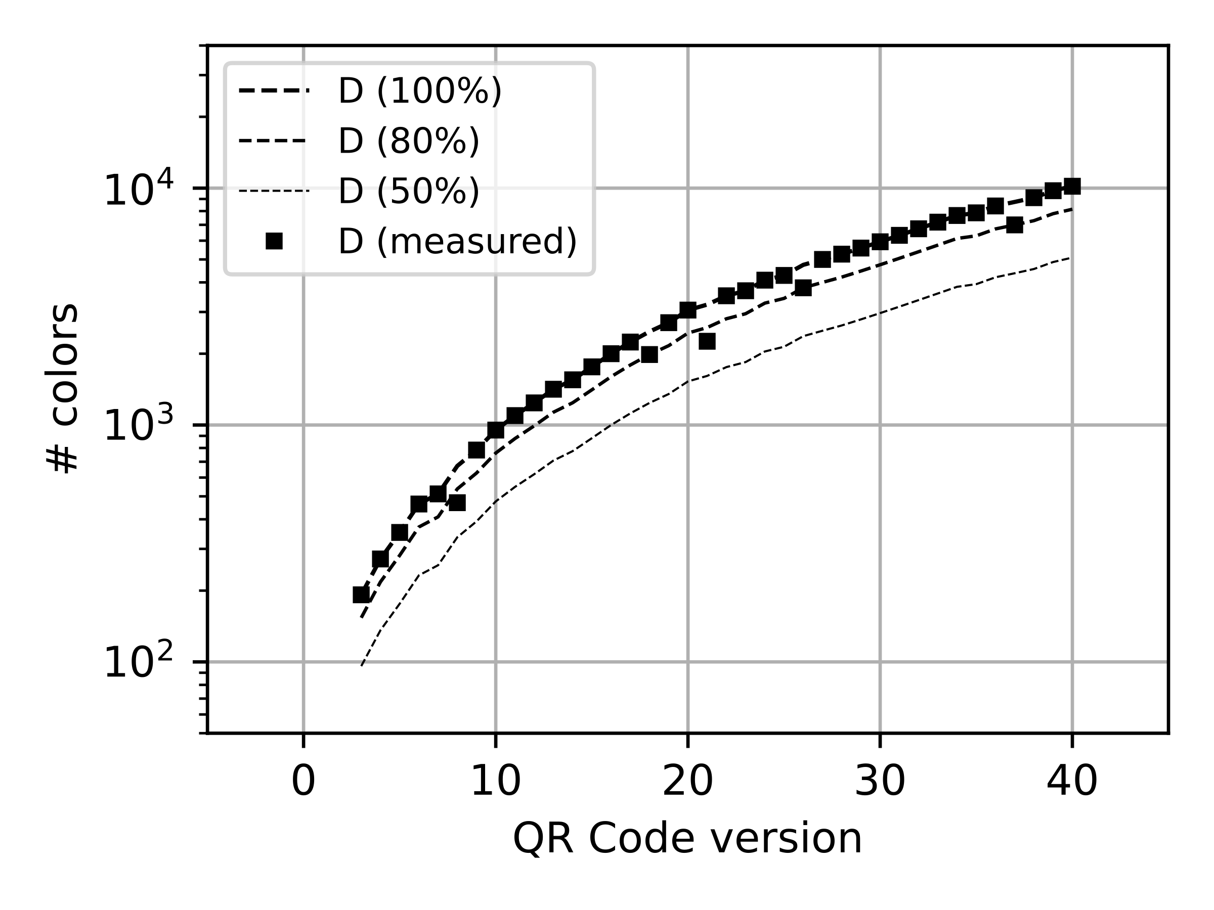
Finally, we illustrate how this approach can be applied to carry out actual color correction problems with full QR Code back-compatibility, using the 24 colors from the original ColorChecker [13] to create a barcode that contains them (see [fig:qrproposal]). We created a compact color QR Code version 5 with H error correction level. According to our findings, this setup should let us embed 352 colors in the data zone (\(Z_D\)) zone without risking readability. In this example, this allowed us to embed up to 10 replicas of the 24 color references, offering plenty of redundancy to detect variations of the color calibrations across the image or to improve the correction itself. Table 5 shows the main quantitative results obtained with this colored QR Code, submitted to the conditions of Experiment 2, with one empty channel and 120.000 image augmentation channels.
| Encoding | ||||
|---|---|---|---|---|
| Digital ID | \(\mathrm{000}\) | |||
| Version | \(\mathrm{5}\) | |||
| Error correction level | H | |||
| Unique colors | \(\mathrm{24}\) | colors | ||
| Total embedded colors | \(\mathrm{240}\) | colors | ||
| Color substitution ratio | \(\mathrm{22}\) | % | ||
| Empty channel | \(\mathrm{1}\) | channel | ||
| SNR | \(\mathrm{12.68}\) | dB | ||
| BER | \(\mathrm{0.0}\) | % | ||
| Success ratio | \(\mathrm{100}\) | % | ||
| Augmentation channels | \(\mathrm{120000}\) | channels | ||
| SNR | \(\mathrm{11 \pm 2}\) | dB | ||
| BER | \(\mathrm{2.7 \pm 1.7}\) | % | ||
| Success ratio | \(\mathrm{96}\) | % |

We have presented a method to pack a set of colors, useful for color calibration, in a QR Code in a fully back-compatible manner; this is, preserving its conventional ability to store digital data. By doing so, we enhanced the state-of-the-art color charts with two main features: first, we did leverage the computer vision readout of the color references to the QR Code features; and two, de facto we reduced the size of the color charts to the usual size of a QR Code, one or two inches.
Also, we have demonstrated that the color capacity of the QR Codes constructed this way (up to a few thousand colors!) is orders of magnitude higher than that found in the traditional color charts, due to the image density and pattern recognition robustness of the QR Codes.
Moreover, compared to other colored QR Codes, our proposal, based on the grayscale affinity of the colors to white or black, leads to much lower signal alteration levels and thus much higher readability, than the found in more naive approaches like, e.g., random assignment methods, which represent the aesthetic QR Codes (printing a logo).
This work opens a way to explore further methods to embed color information in conventional 2D barcodes. Tuning how we defined our criteria of color embedding upon the affinity of colors to black and white would lead to more efficient embedding methods. We explored some of these ideas to seek those improved methods, and we expose them below.
First, the way in which we implemented the grayscale (a mean value of the RGB channels) is only one of the ways to compute a grayscale channel. For example, one could use the luma definition a weighted mean based on the human eye vision:
\[f_{grasycale}(r, g, b) = 0.2126\cdot r + 0.7152\cdot g + 0.0722\cdot b \ ,\]
or the lightness one:
\[f_{grasycale}(r, g, b) = \frac{1}{2} \left( \max(r, g, b) + \min(r, g, b) \right) \ .\]
These grayscale definitions are often part of colorspaces definitions [11], such as CIELab, CIELuv, HSL, etc. All these different grayscales will generate different color distributions, displacing colors between black and white regions of the QR Code.
Second, we defined a way to select the area inside the QR Code to embed the colors (see [algorithm]), that could also be improved. For example, we could decide to implement \(f_{threshold}\) in a more complex fashion. Let us imagine a certain set of colors \(G_{rgb}\) to encode in a certain QR Code. One could create more than two subsets to define the black-white affinity, i.e. four sets, namely: blackest colors (0), blackish colors (1), whitish colors (2) and whitest colors (3):
\[f_{threshold}(G_{gray}) = \begin{cases} 0 & 0.00 < G_{gray}(k) \leq 0.25 \\ 1 & 0.25 < G_{gray}(k) \leq 0.50 \\ 2 & 0.50 < G_{gray}(k) \leq 0.75 \\ 3 & 0.75 < G_{gray}(k) \leq 1.00 \\ \end{cases}\]
And accommodate [algorithm] to this new output from \(f_{grayscale}\) by assigning those colors with higher potential error (\(\mathrm{1, \ 2}\)) to the DATA zone and those with lower potential error (\(\mathrm{0, \ 3}\)) to the EC zone. Theoretically, this would outperform our current approach, as in this work we demonstrated that DATA zones are more resilient to error than EC zones, thus displacing away from EC critical colors would lead to a systematic increase of color capacity.
Third, many authors have contributed to create aesthetic QR Codes which embed trademarks and images with incredibly detailed results. We wanted to highlight some solutions that might be combined with our technology to embed even further colors or to improve the control over the placement of the colors.
Halftone QR Codes were proposed by Chu et al. [56], they substituted QR Code modules for subsampled modules that contained white and black colors (see [fig:qrswithlogos]). These submodules presented a dithering pattern that followed the encoded image shape. One could use the dithering idea to embed also colors inside subsampled pixels.
QArt Codes were introduced by Cox [58], the proposal aims to force the QR Code encoding to block certain areas of the QR Code to be black or white no matter what the encoded data is, note this is only possible for some kinds of data encoding (see [fig:qrswithlogoscolor]). One could use this feature to preserve dedicated areas for color embeddings, as a complement to [algorithm]. Note that the need for a back-compatible criteria is still-present, since the QArt Code only provides us the certainty if a module of the original QR Code is black or white, but they must remain black or white during the decoding process. This has a potential impact in reducing the cost of producing the Color QR Codes, because one could fix the position of the colored modules before encoding the data using our grayscale criteria, then print the QR Code using cost-effective printing technologies (rotogravure, flexography, etc.) and the black and white pixels using also cost-effective monochromatic printing technologies (laser printing), rather than using full digital ink-jet printing to print the whole code.
Finally, we have assumed that our back-compatible Color QR Codes are meant to be for colorimetric measurement, as this is the preamble of our research.
Nevertheless, the above-presented results could be applied to encode data in the color of the QR Codes in a back-compatible manner. This means, including more digital information in the same space. Other authors have presented their approaches to this solution, none of them in a back-compatible way. Les us propose a couple of ideas to achieve these digital back-compatible Color QR Codes, based on other ideas to color encode data in QR Codes.
First, Blasinki et al. [130] introduced a way to multiplex 3 QR Codes in one, by encoding a QR Code in each CMY channel of the printed image. And then, when they recovered the QR Code, they applied a color interference cancellation algorithm to extract the QR Codes from the RGB captured image, they also discussed how to approach the color reproduction problem and manipulated further the remaining black patterns (finder, alignment and timing) to include color references.
All in all, this rendered non back-compatible Color QR Codes. Now, using our proposed method, one could turn this approach to back-compatibility again by simply doing the following: keeping the first QR Code to multiplex as the ’default’ QR Code; then, taking another 3 additional QR Codes and creating a barcode following Blasinki et al. method; in turn, creating a "pseudo-white" and "pseudo-black" version of this color QR Code; and finally, re-encoding the default QR Code with the pseudo-colors in a back-compatible manner. Also, note that this proposal is not restricted by the number of channels an image has, as we are exploiting intermediate values, not only the extreme ones. There should exist a limit yet to discover of how many QR Code can be multiplexed in this fashion.
Second, other authors like Berchtold et al. – JAB Code (see [fig:2dbarcodes]) [49] or Grillo et al. – HCCBC (see [fig:othercolorqrs]) [133] fled from the original QR Code standard to redefine entirely the data encoding process. The main caveat of their technological proposals is the lack of back-compatibility, as we have discussed before. One could combine both technologies to create more adoptable technology. Grillo et al. proposal seems the easiest way to go, as they kept the factor form of QR Codes. Theoretically, one could simply multiplex one HCCBC with one QR Code as described with the previous method and achieve a digital back-compatible Color QR Code.
Thin-plates splines (TPS) were introduced by Duchon in 1978 [137], and reformulated by Meinguet in 1979 [138]. Later in 1989, TPS were popularized by Bookestein [115] due to their potential to fit data linked by an elastic deformation, especially when it comes to shape deformation.
So far, TPS have been used widely to solve problems like morphing transformations in 2D spaces. For example, Rohr et al. [139] and Crum et al. [140] used TPS to perform elastic registration of similar features in different images in a dataset. Or, Bazen et al. [116] used TPS to match fingerprints. Moreover, we have successfully used TPS to improve QR Code extraction in [ch:4].
The TPS framework can be applied to color spaces. As explained in [ch:3], color spaces are three-dimensional spaces. The TPS formulation covers this scenario for 3D deformations [115], [137], [138]. In fact, we can already find works that apply them to color technology. For example, Colatoni et al. [141] and Poljicak et al. [142] used TPS to characterize screen displays. Also, Sharma et al. [143] interpolated colors to be printed in commercial printers using TPS. Moreover, Menesatti et al. [15] proposed a new approach to color correct dataset for image consistency based upon TPS, and called this method 3D Thin-Plate Splines (TPS3D).
In this chapter, we focus on the implementation of thin-plate spline color corrections, specifically in the use of the TPS3D method to perform color correction in image datasets directly in RGB spaces, while proposing an alternative radial basis function [144] to be used to compute the TPS, and introducing a smoothing factor to approximate the solution in order to reduce corner-case errors [145]. All in all, we illustrate here the advantages and limitations of the new TPS3D methodology to color correct RGB images.
Solving the image consistency problem, introduced in [ch:3], using the TPS3D method requires the creation of an image dataset. The images on this dataset must contain some type of color chart. Also, the captured scenes in the images must be meaningful, and the color chart must be representative of those scenes. Here, we propose to use the widely-accepted Gehler’s ColorChecker dataset [146], [147], which contains 569 images with a 24 patch Macbeth ColorChecker placed in different scenes (see [fig:gehler_example]). We do so, rather than creating our own dataset with the Back-compatible Color QR Codes proposed in [ch:5] because this is a standard dataset with a standard color chart. In [ch:7], we will combine both techniques into a colorimetric sensor.
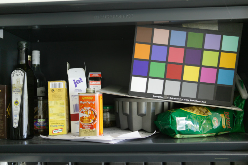
Moreover, we propose to apply a data augmentation technique to increase the size of the dataset by 100, to match in size other augmented image datasets that have appeared recently. We do not use those images as they do not always contain a ColorChecker [12].
Furthermore, we propose to benchmark our TPS3D against its former implementation [15] and a range of alternative methods to correct the color in images, such as: white balance [44], affine [44], polynomial [27], [28] and root-polynomial [28] corrections. Benchmarking includes both quantitative color consistency and computational cost metrics [15], [148].
In the following we review the derivation of the above-mentioned color correction methods before introducing our improvements to the TPS3D method. Notice the formulation will remind to the 2D projection formulation from [ch:4], however some differences have to be considered:
as described in [ch:3], color corrections are mappings between 3D spaces,
unlike projective transformations in 2D planes, we will only be using affine terms as basis, and
our notation in this formulation avoids the use of homogeneous coordinates \((p_0, p_1, p_2)\) in favor of more verbose notation using the name of each color channel \((r, g, b)\).
In [ch:3] we defined color corrections as an application \(f\) between two RGB color spaces. If this application is to be linear, thus a linear correction, we can use a matrix product notation to define the correction [14], [44]:
\[\mathbf{s}' = f(\mathbf{s}) = \mathbf{M} \cdot \mathbf{s}\]
where \(\mathbf{M}\) is a 3 \(\times\) 3 linear matrix that maps each color in the origin captured color space \(\mathbf{s} = (r, g, b)\) to the corrected color space \(\mathbf{s}' = (r', g', b')\) (see [fig:NONE]). In order to solve this system of equations, we must substitute these vectors by matrices containing enough color landmarks (known pairs of colors in both spaces) to solve the system for \(\mathbf{M}\):
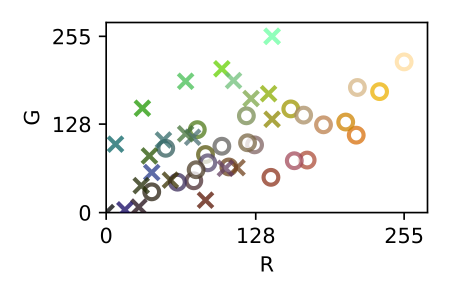
\[\mathbf{M} \cdot \mathbf{P} = \mathbf{Q} \label{eq:MPQ}\]
where \(\mathbf{Q}\) is matrix with \(\mathbf{s}'\) colors and \(\mathbf{P}\) is matrix with \(\mathbf{s}\) colors.
White-balance is the simplest color transformation that can be applied to an RGB color. In the white-balance correction each channel of vector function \(f\) is independent:
\[\begin{split} r' &= f_r (r) = \frac{r_{max}}{r_{white}} \cdot r \\ g' &= f_g (g) = \frac{g_{max}}{g_{white}} \cdot g \\ b' &= f_b (b) = \frac{b_{max}}{b_{white}} \cdot b \end{split} \label{eq:whitebalance}\]
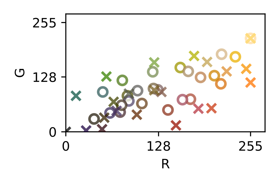
where \((r_{max}, g_{max}, b_{max})\) is the maximum value of each channel in the color corrected space, e.g. \((255, 255, 255)\) for 24-bit images; and \((r_{white}, g_{white}, b_{white})\) is the measured whitest color in the image (see [fig:AFF0]). This relation can be easily written as a matrix, and only needs one color reference to be solved (from [eq:MPQ]):
\[\begin{pmatrix} a_r & 0 & 0 \\ 0 & a_g & 0 \\ 0 & 0 & a_b \end{pmatrix} \cdot \begin{pmatrix} r \\ g \\ b \end{pmatrix} = \begin{pmatrix} r' \\ g' \\ b' \end{pmatrix}\]
where \(a_k\) are the weight contributions of [eq:whitebalance] for each \(k\) channel.
The white-balance correction can be improved by subtracting the black level of the image before applying the white-balance correction (see [fig:AFF1]). For example, this improvement looks like (shown for the red channel for simplicity):
\[r' = f_r (r) = r_{min} + \frac{r_{max} - r_{min}}{r_{white} - r_{black}} \cdot (r - r_{black}) \label{eq:whitebalanceblacksubtraction}\]
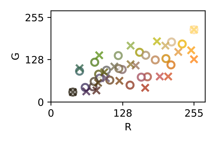
where \(r_{min}\) is the minimum value of the channel red possible in the color corrected space, e.g. 0 for 24-bit images; and \(r_{black}\) is the red value of the measured darkest color in the image. [eq:MPQ] is still valid for this linear mapping, but \(f\) becomes a composed application (\(f: \mathbb{R}^3 \to \mathbb{R}^4 \to \mathbb{R}^3\)), where \(\mathbf{M}\) becomes a 3 \(\times\) 4 matrix, and we need to expand the definition of the \(\mathbf{P}\) colors using a homogeneous coordinate:
\[\begin{pmatrix} a_r & 0 & 0 & t_r \\ 0 & a_g & 0 & t_g \\ 0 & 0 & a_b & t_b \end{pmatrix} \cdot \begin{pmatrix} r_1 & r_2 \\ g_1 & g_2 \\ b_1 & b_2 \\ 1 & 1 \end{pmatrix} = \begin{pmatrix} r'_1 & r'_2 \\ g'_1 & g'_2 \\ b'_1 & b'_2 \end{pmatrix}\]
where \(a_k\) are the affine contributions and \(t_k\) are the translation contributions for each \(k\) channel, and now two points are required to obtain the color correction weights.
White balance is only a particular solution of an affine correction. We can generalize [eq:whitebalance] for, e.g., the red channel to accept contributions from green and blue channels:
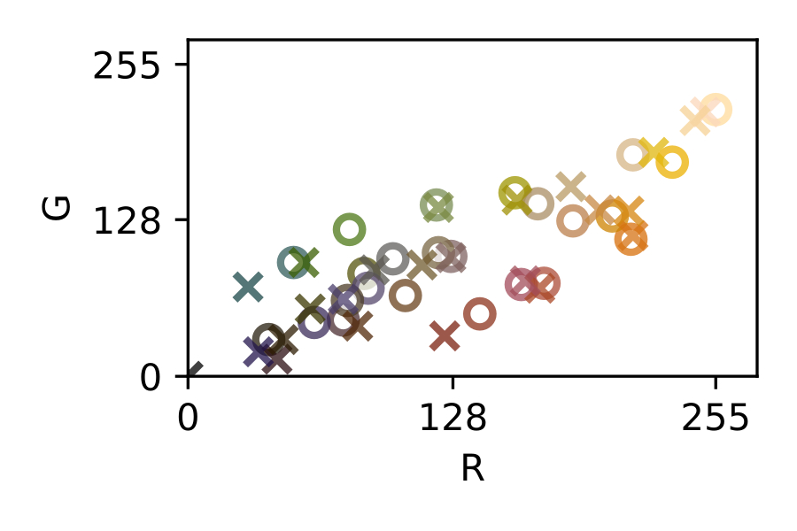
\[r' = f_r (r, g, b) = a_{r, r} \cdot r + a_{r, g} \cdot g + a_{r, b} \cdot b = \sum_k^{r,g,b} a_{r, k} k\]
this expression is connected with the full matrix implementation, with 9 unknown weights:
\[\begin{pmatrix} a_{r,r} & a_{r,g} & a_{r,b} \\ a_{g,r} & a_{g,g} & a_{g,b} \\ a_{b,r} & a_{b,g} & a_{b,b} \end{pmatrix}\cdot \begin{pmatrix} r_1 & r_2 & r_3 \\ g_1 & g_2 & g_3 \\ b_1 & b_2 & b_3 \\ 1 & 1 & 1 \end{pmatrix} = \begin{pmatrix} r'_1 & r'_2 & r'_3 \\ g'_1 & g'_2 & g'_3 \\ b'_1 & b'_2 & b'_3 \end{pmatrix}\]
where \(a_{j,k}\) are the weights of the \(\mathbf{M}\) matrix, and we need 3 known colors references to solve the system (see [fig:AFF2]).
In turn, white-balance with black-subtraction [eq:whitebalanceblacksubtraction] is a specific solution of an affine transformation, which handles translation and can be generalized as:

\[r' = f_r (r, g, b) = t_r + \sum_k^{r,g,b} a_{r, k} k \label{eq:affine}\]
also tied up to its matrix representation:
\[\begin{pmatrix} a_{r,r} & a_{r,g} & a_{r,b} & t_r \\ a_{g,r} & a_{g,g} & a_{g,b} & t_g \\ a_{b,r} & a_{b,g} & a_{b,b} & t_b \end{pmatrix} \cdot \begin{pmatrix} r_1 & r_2 & r_3 & r_4 \\ g_1 & g_2 & g_3 & g_4 \\ b_1 & b_2 & b_3 & b_4 \\ 1 & 1 & 1 & 1 \end{pmatrix} = \begin{pmatrix} r'_1 & r'_2 & r'_3 & r'_4 \\ g'_1 & g'_2 & g'_3 & g'_4 \\ b'_1 & b'_2 & b'_3 & b'_4 \end{pmatrix}\]
where \(a_{j,k}\) and \(t_k\) are the weights of the \(\mathbf{M}\) matrix, and we require 4 known colors to solve the system (see [fig:AFF3]).
As we have seen with affine corrections, we can expand the definition of the measured color space matrix \(\mathbf{P}\) including additional terms to it. This is useful to compute non-linear corrections using a linear matrix implementation. Formally, this space expansion can be seen as \(f\) being now a composed application:
\[f: \mathbb{R}^3 \rightarrow \mathbb{R}^{3+N} \rightarrow \mathbb{R}^3\]
where \(\mathbb{R}^{3+N}\) is an extended color space derived from the original color space \(\mathbb{R}^3\). We can write a generalization of [eq:affine] for polynomial corrections as follows:
\[r' = f_r (r, g, b) = t_r + \sum_k^{r,g,b} a_{r, k} k + \sum_i^N w_{r,i} \Phi_i (r, g, b) \label{eq:polynomial}\]
where \(\Phi (r,g,b) = \{\Phi_i (r,g,b) \}, \ i=1,\cdots,N\) is a set of monomials, \(w_i\) are the weight contributions for each monomial and \(N\) is the length of the monomial set [28].
The monomials in the set \(\Phi (r,g,b)\) will have a degree 2 or more, because we do not unify the affine parts as monomials, we do so to emphasize their contribution to the correction. Also, notice that \(N\) is arbitrary, and we can choose how we construct our polynomial expansions by tuning the monomial generator \(\Phi_i (r, g, b)\).
Despite that, \(N\) always relates to the number of vectors needed in [eq:MPQ] to solve the system. \(\mathbf{M}\) takes the form of a \(3 \times (4+N)\) matrix, \(\mathbf{P}\) takes the form of a \((4 + N) \times (4 + N)\) matrix and \(\mathbf{Q}\) takes the form of a \(3 \times (4 + N)\) :
\[\begin{pmatrix} w_{r,N} & \cdots & w_{r,1} & a_{r,r} & a_{r,g} & a_{r,b} & t_r \\ w_{g,N} & \cdots & w_{g,1} & a_{g,r} & a_{g,g} & a_{g,b} & t_g \\ w_{b,N} & \cdots & w_{b,1} & a_{b,r} & a_{b,g} & a_{b, b} & t_b \end{pmatrix} \cdot \begin{pmatrix} \Phi_{N,0} & \Phi_{N,2} & \dots & \Phi_{N,N+4} \\ \vdots & \vdots & \vdots & \vdots \\ \Phi_{1,1} & \Phi_{1,2} & \dots & \Phi_{1, N+4} \\ r_1 & r_2 & \dots & r_{N+4} \\ g_1 & g_2 & \dots & g_{N+4} \\ b_1 & b_2 & \dots & b_{N+4} \\ 1 & 1 & \dots & 1 \end{pmatrix} = \begin{pmatrix} r'_1 & r'_2 & \dots & r'_{N+4} \\ g'_1 & g'_1 & \dots & g'_{N+4} \\ b'_1 & b'_1 & \dots & b'_{N+4} \end{pmatrix} \label{eq:polynomialmatrix}\]
The simplest polynomial expansion of a color space occurs when \(\Phi (r, g, b)\) generates a pure geometric set:
\[\Phi (r, g, b) = \left\{k^\upalpha : \ 2 \leq \upalpha \leq D \right\} \label{eq:polyset0}\]
where \(k \in \{r, g, b\}\) is any of the RGB channels, \(\upalpha\) is the degree of a given monomial of the set and \(D\) is the maximum degree we choose to form this set (see [fig:VAN2]). For example, for \(D = 3\) , it will produce the set:
\[\Phi_{D=3} (r, g, b) = \left\{r^2, \ g^2, \ b^2, \ r^3, \ g^3, \ b^3 \ \right\}\]
Combining this expression with [eq:polynomialmatrix], we can see we obtain a matrix that is directly related with the Vandermonde matrix [149], but for 3D data instead of 1D data.

[eq:polyset0] can be generalized to take into account also cross-terms from any of the channels to create the monomial terms [27], [28]. So, we can write now:
\[\Phi (r, g, b) = \left\{\prod_k^{rgb} k^{\upalpha_k} \ : \ 2 \leq | \upalpha | \leq D \right\} \label{eq:polyset1}\]
where \(| \upalpha | = \sum_k^{rgb} \upalpha_k\) is a metric, which is the sum of the degrees of each channel in the monomial, thus the degree of each monomial.
Following with the example where \(D = 3\), now we obtain an expanded set:
\[\Phi_{D=3} (r, g, b) = \left\{r^2, \ g^2, \ b^2, \ rg, \ gb, \ br, \ r^3, \ g^3, \ b^3, \ rg^2, \ gb^2, \ br^2, \ gr^2, \ bg^2, \ rb^2, \ rgb \right\}\]
Finally, a root-polynomial correction is defined modifying [eq:polyset1] to introduce the \(| \upalpha |\)-th root to each monomial [28]:
\[\Phi (r, g, b) = \left\{\prod_k^{rgb} k^{\frac{\upalpha_k}{| \upalpha|}} \ : \ 2 \leq | \upalpha | \leq D \right\}\]
So, this reduces the amount of terms of each set for a given degree \(D\). Then, our example with \(D= 3\) becomes reduced to:
\[\Phi_{D=3} (r, g, b) = \left\{\sqrt{rg}, \sqrt{gb}, \sqrt{br}, \sqrt[3]{rg^2}, \sqrt[3]{gb^2}, \sqrt[3]{br^2}, \sqrt[3]{gr^2}, \sqrt[3]{bg^2}, \sqrt[3]{rb^2}, \sqrt[3]{rgb} \right\}\]
Notice that all the terms present in a Vandermonde expansion have now disappeared, as they are now the same terms of the affine transformation due to the root application \(\{\sqrt[3]{r^3}, \sqrt[3]{g^3}, \sqrt[3]{b^3}\} = \{\sqrt{r^2}, \sqrt{g^2}, \sqrt{b^2}\} = \{r, g, b\}\), and the only remaining terms are the roots of the cross-products.
As an alternative to the former approaches, we can use thin-plate spline as the basis of the expansion to the color space in \(\mathbf{P}\) [15]:
\[r' = f_r (r, g, b) = t_r + \sum_k^{r,g,b} a_{r, k} k + \sum_i^N w_{r,i} h_i (r, g, b) \label{eq:thinplate}\]

where \(w_i\) are the weight contributions for each spline contributions, and \(h_i (r, g, b)\) are kernels of \(h\) in the \(N\) known colors. We will follow the same formulation described in [ch:4]. A more detailed definition of \(h_i\) functions can be found there. Also, notice that this expression is really similar to [eq:polynomial] of polynomial corrections, the main difference is the fact that the number of \(N\) spline contributions equals to the number of color references (see [fig:TPS1]).
[eq:MPQ] becomes now:
\[\begin{pmatrix} w_{r,1} & \cdots & w_{r,N} & a_{r,r} & a_{r,g} & a_{r,b} & t_r \\ w_{g,1} & \cdots & w_{g,N} & a_{g,r} & a_{g,g} & a_{g,b} & t_g \\ w_{b,1} & \cdots & w_{b,N} & a_{b,r} & a_{b,g} & a_{b, b} & t_b \end{pmatrix} \cdot \begin{pmatrix} h_{1,1} & h_{1,2} & \dots & h_{1,N} \\ \vdots & \vdots & \vdots & \vdots \\ h_{N,1} & h_{N,2} & \dots & h_{N, N} \\ r_1 & r_2 & \dots & r_{N} \\ g_1 & g_2 & \dots & g_{N} \\ b_1 & b_2 & \dots & b_{N} \\ 1 & 1 & \dots & 1 \end{pmatrix} = \begin{pmatrix} r'_1 & r'_2 & \dots & r'_{N} \\ g'_1 & g'_1 & \dots & g'_{N} \\ b'_1 & b'_1 & \dots & b'_{N} \end{pmatrix} \label{eq:thinplatematrix}\]
This system is unbalanced, as we have \(N\) colors vectors in \(\mathbf{P}\) and \(\mathbf{Q}\). In other corrections, we used four additional color references to solve the system, but here each new color is used to compute an additional spline, unbalancing the system again. Alternatively, the TPS formulation imposes two additional conditions [115]: the sum of \(w_{j,k}\) coefficients is to be \(\mathrm{0}\), and their cross-product with the \(\mathbf{P}\) colors as well. As a consequence of such conditions, spline contributions tend to \(\mathrm{0}\) at infinity, while affine contributions prevail. This makes our system of equations solvable, and it can be expressed as an additional matrix product:
\[\begin{pmatrix} w_{r,1} & \cdots & w_{r,N} \\ w_{g,1} & \cdots & w_{g,N} \\ w_{b,1} & \cdots & w_{b,N} \end{pmatrix} \cdot \begin{pmatrix} r_1 & ... & r_N \\ g_1 & ... & g_N \\ b_1 & ... & b_N \\ 1 & ... & 1 \end{pmatrix}^T = 0\]
The radial basis functions (RBF) used to compute splines remains open to multiple definitions. The thin-plate approach to compute those splines implies using solutions of the biharmonic equation [115]:
\[\Delta^{2} U = 0\]
that minimize the bending energy functional described by many authors, thus resembling the spline solution to the trajectory followed by an n-dimensional elastic plate. These solutions are the polynomial radial basis functions and a general solution is provided for n-dimensional data as [139], [144], [145]:
\[h_c(\mathbf{s}) = U(\mathbf{s}, \mathbf{c}) = \begin{cases} || \mathbf{s} - \mathbf{c} ||^{2k-n} \ln|| \mathbf{s} - \mathbf{c} || & 2k-n \text{ is even} \\ || \mathbf{s} - \mathbf{c} ||^{2k-n} & \text{otherwise} \end{cases}\]
where \(n\) is the number of dimensions, \(k\) is the order of the functional, \(\mathbf{s}\) and \(\mathbf{c}\) are the data points where the spline is computed and \(|| \cdot ||\) is a metric.
For a bending energy functional (the metal thin-plate approach) \(k = 2\) and \(n = 2\) (2D data), we obtain the usual thin-plate spline RBF [115]:
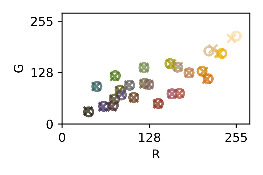
\[h_c(\mathbf{s}) = || \mathbf{s} - \mathbf{c} ||^2 \ln|| \mathbf{s} - \mathbf{c} || \label{eq:rbf2D}\]
But for \(k = 2\) and \(n = 3\) (3D data) we obtain [115]:
\[h_c(\mathbf{s}) = || \mathbf{s} - \mathbf{c} || \label{eq:rbf3D}\]
It is unclear why in the TPS3D to color correct images, Menesatti et al. [15] used the definition for 2D data ([eq:rbf2D]), rather than the actual 3D definition ([eq:rbf3D]) which according to the literature should yield to more accurate results. We will investigate here the impact of this change in the formal definition of the TPS3D.
So far, we have not defined a metric \(|| \cdot ||\) to solve the TPS contributions. We will follow Menesatti et al. and use the euclidean metric of the RGB space. We will also name this metric \(\Delta_{RGB}\), as it is commonly known in colorimetry literature [15]:
\[|| \mathbf{s} - \mathbf{c} || = \Delta_{RGB}(\mathbf{s}, \mathbf{c}) = \sqrt{(r_s - r_c)^2 + (g_s - g_c)^2 + (b_s - b_c)^2} \label{eq:rgb_distance}\]
Approximating the TPS corrections is a well-known technique [139], [145]. Specifically, this is performed in ill-conditioned scenarios where data is noisy or saturated, and strict interpolation between data points, leads to important error artifacts. We propose now adding a smoothing factor to the TPS3D, to improve color correction in ill-conditioned situations.
We approximated the TPS by adding a smoothing factor to the spline contributions, which reduces the spline contributions in favor of the affine ones (see [fig:TPS3]). Taking [eq:thinplate], we will introduce a smooth factor only for those color references where the center of the spline was those references themselves:
\[r'_j = f_r (r_j, g_j, b_j) = t_r + \sum_k^{r_j,g_j,b_j} a_{r, k} k + \sum_i^N ( w_{r,i} h_i (r_j, g_j, b_j) + \lambda \delta_{ij})\]
where \(\lambda\) is the smoothing factor, and \(\delta_{ij}\) is a Kronecker delta.
Notice that in the previous TPS definition the spline contributions of a reference color to the same reference color were \(\mathrm{0}\) under the euclidean metric we chose. Also, notice that the matrix product of [eq:thinplatematrix] is still valid, as we have only affected the diagonal of the upper part of the \(\mathbf{P}\) matrix. Thus,
\[\mathbf{P}_{smooth} = \mathbf{P} + \begin{bmatrix} \lambda \mathbf{I} \\ \mathbf{O}(4,N) \end{bmatrix} = \begin{pmatrix} h_{1,1} + \lambda & h_{1,2} & \dots & h_{1,N} \\ h_{2,1} & h_{2,2} + \lambda & \dots & h_{2,N} \\ \vdots & \vdots & \vdots & \vdots \\ h_{N,1} & h_{N,2} & \dots & h_{N, N} + \lambda \\ r_1 & r_2 & \dots & r_{N} \\ g_1 & g_2 & \dots & g_{N} \\ b_1 & b_2 & \dots & b_{N} \\ 1 & 1 & \dots & 1 \end{pmatrix}\]
where \(\mathbf{P}\) is the matrix of color references and their TPS expansion, \(\mathbf{I}\) is the identity matrix and \(\mathbf{O} (4, N)\) is a matrix with \(\mathrm{0}\)s of size \(4 \times N\).
So far, we have reviewed the state-of-the-art methods to color correct images to achieve consistent datasets using color references as fixed points in color spaces to compute color corrections. Also, we have proposed two updates to the TPS3D method: using the suited RBF and smoothing the TPS contributions.
In Table 1, we show a summary of all the corrections that we studied in this work using the dataset described in the next section. First, a perfect correction (PERF) and a non-correction (NONE) scenario are present as reference. Notice that perfect correction will display here the quantization error after passing from 12-bit images to 8-bit images. Then, several corrections have been implemented, that have been grouped by authorship of the methods and type of correction:
Affine (AFF): white-balance (AFF0), white-balance with black subtraction (AFF1), affine (AFF2), affine with translation (AFF3).
Vandermonde (VAN): four polynomial corrections from degree 2 to 5 (VAN0, VAN1, VAN2 and VAN3).
Cheung (CHE): from Cheung et al. [27], four polynomial corrections with different terms: 5 (CHE0), 7 (CHE1), 8 (CHE2) and 10 (CHE3).
Finlayson (FIN): from Finlayson et al. [28], two polynomial and two root-polynomial, of degrees 2 and 3 (FIN0, FIN1, FIN2, FIN3).
Thin-plate splines (TPS): TPS3D from Menesatti et al. [15] (TPS0), our method using the proper RBF (TPS1) and the same method with two smoothing values (TPS2 and TPS3).
| Correction | Acronym | \(\mathbf{P}\) extended color space |
|---|---|---|
| Perfect | PERF | \((r, g, b)\) |
| No correction | NONE | \((r, g, b)\) |
| White-balance | AFF0 | \((r, g, b)\) |
| White-balance w/ black subtraction | AFF1 | \((1, r, g, b)\) |
| Affine | AFF2 | \((r, g, b)\) |
| Affine w/ translation | AFF3 | \((1, r, g, b)\) |
| Vandermonde (degree=2) | VAN0 | \((1, r, g, b, r ^2, g ^2, b ^2)\) |
| Vandermonde (degree=3) | VAN1 | \((1, r, g, b, r ^2, g ^2, b ^2, r ^3, g ^3, b ^3 )\) |
| Vandermonde (degree=3) | VAN2 | \((1, r, g, b, r ^2, g ^2, b ^2, r ^3, g ^3, b ^3, r ^4, g ^4, b ^4 )\) |
| Vandermonde (degree=4) | VAN3 | \((1, r, g, b, r ^2, g ^2, b ^2, r ^3, g ^3, b ^3, r ^4, g ^4, b ^4, r ^5, g ^5, b ^5)\) |
| Cheung (terms=5) | CHE0 | \((1, r, g, b, rgb)\) |
| Cheung (terms=7) | CHE1 | \((1, r, g, b, rg, rb, gb)\) |
| Cheung (terms=8) | CHE2 | \((1, r, g, b, rg, rb, gb, rgb)\) |
| Cheung (terms=10) | CHE3 | \((1, r, g, b, rg, rb, gb, r ^2, g ^2, b ^2)\) |
| Finlayson (degree=2) | FIN0 | \((r, g, b, r ^2, g ^2, b ^2, rg, rb, gb)\) |
| Finlayson (degree=3) | FIN1 | \((r, g, b, r ^2, g ^2, b ^2, rg, rb, gb, r ^3, g ^3, b ^3,\) |
| \(rg ^2, gb ^2, rb ^2, gr ^2, bg ^2, br ^2, rgb)\) | ||
| Finlayson root (degree=2) | FIN2 | \((r, g, b, \sqrt{rg}, \sqrt{rb}, \sqrt{gb})\) |
| Finlayson root (degree=3) | FIN3 | \((r, g, b, \sqrt{rg}, \sqrt{rb}, \sqrt{gb}, \sqrt[3]{rg ^2}, \sqrt[3]{gb ^2}, \sqrt[3]{rb ^2},\) |
| \(\sqrt[3]{gr ^2}, \sqrt[3]{bg ^2}, \sqrt[3]{br ^2}, \sqrt[3]{rgb})\) | ||
| Thin-plate splines (Manesatti) | TPS0 | \((1, r, g, b, \Delta_1 ^2 \ln \Delta_1, \dots, \Delta_{24} ^2 \ln \Delta_{24})\) |
| Thin-plate splines (ours, smooth=0) | TPS1 | \((1, r, g, b, \Delta_1, \dots, \Delta_{24})\) |
| Thin-plate splines (ours, smooth=0.001) | TPS2 | \((1, r, g, b, \Delta_1, \dots, \Delta_{24})\) |
| Thin-plate splines (ours, smooth=0.1) | TPS3 | \((1, r, g, b, \Delta_1, \dots, \Delta_{24})\) |
As explained before, the usual approach to solve the image consistency problem is placing color references in a certain scene to later perform a color correction. There exists a widely spread usage of color charts, e.g. Macbeth ColorChecker of 24 colors [13]. Over the years, extensions of this ColorChecker have appeared, mostly presented by X-Rite, a Pantone company, or by Pantone itself, which introduced the Pantone Color Match Card that features four AruCo patterns [19] to ease the pattern extraction when acquiring the colors of the chart.
Since in this chapter we do not propose improved versions of the charts themselves, we use an existing image dataset that contains images of the Macbeth ColorChecker of 24 colors in different scenes in order to evaluate our color correction with respect to image consistency; and benchmark it against other correction methods. The Gehler’s dataset is a widely used dataset with several versions, and there exists a deep discussion about how to use it. Despite the efforts of the dataset creators and other authors to promote the use of the last “developed” dataset [147], here we use the RAW original version of the dataset [146], and we developed the images ourselves. We did so because we performed image augmentation over the dataset, as we want to control the developing process of the RAW images and also measuring the resulting augmented colors directly from the provided annotations in the original dataset (see [fig:ccdatasetpipeline]).
![Our pipeline: for each Gehler’s dataset raw image (Bayer) we developed an RGB image, which are already the half size of the original image, also this image was down-sampled to reduce its size 4 times. Then we augmented this down-sampled image with 100 sample augmentation scenarios. For each augmented scenario we corrected it back before augmentation using the 21 different correction methods described in [tab:correctionssummary].](assets/graphics/chapters/chapter6/figures/cc_dataset_pipeline.jpg)
The Gehler’s dataset comprises images from two cameras: a Canon EOS 1DS (86 images) and a Canon EOS 5D (483 images), both cameras producing raw images of 12-bit per channel (\(\mathbb{N}^3_{[0, 4096]}\)) with a RGGB Bayer pattern [150]. This means we have twice as many green pixels than red or blue pixels.
Images have been processed using Python [151], represented by
numpy arrays [86], [152], and have been
developed using imageio [92] and rawpy, the Python
wrapper of craw binary, the utility used elsewhere to
process the Gehler’s dataset [146], [147]. When developing
the images, we implemented no interpolation, thus rendering images half
the size of the raw image (see [tab:ccdatasetdownsampling]).
These are our ground-truth images: the colors in these images
are what we are trying to recover when performing the color
corrections.
We chose to work with 8-bits per channel RGB images as is the most commonly developed pixel format present nowadays. First, we cast the developed dataset 12-bit images (\(\mathbb{N}^3_{[0, 4096]}\)) to 8-bit resolution (\(\mathbb{N}^3_{[0, 255]}\)). The difference between the cast images and the groundtruth images is the quantization error, due to the loss of color depth resolution. To speeded up the calculations without losing statistical significance in the results we down-sampled the images by a factor 4. The down-sampling factor is arbitrary and depends on the level of redundancy of the color distribution in our samples. We selected a down-sampling factor that did not alter the color histogram of the images of the dataset, see [fig:ccdatasethistogram]. [tab:ccdatasetdownsampling] shows the final image sizes for each camera on the Gehler’s dataset.
| Camera | Raw image | Developed image | Down-sampled image |
|---|---|---|---|
| Canon EOS 1DS | \(\mathrm{(4064,\ 2704)}\) | \(\mathrm{(2041,\ 1359)}\) | \(\mathrm{(511,\ 340)}\) |
| Canon EOS 5D | \(\mathrm{(4368,\ 2912)}\) | \(\mathrm{(2193,\ 1460)}\) | \(\mathrm{(549,\ 365)}\) |
Subsequently, we augmented the dataset using imgaug
[93] (see [fig:ccdatasetaugmentation])
that generated image replicas simulating different acquisition setup
conditions. The augmentations were performed with random augmentations
that modeled: linear contrast, gamma contrast and channel cross-talk.
Geometrical distortions were omitted because this work is focused on a
colorimetry problem.
Finally, we corrected each developed, down-sampled and augmented
image using the color corrections listed in [tab:correctionssummary].
These corrections were computed using color-normalized versions of those
images (\(\mathbb{R}^{3}_{[0, 1]}\)).
White-balance corrections were implemented directly with simple array
operations [86]; while
affine, polynomial and root-polynomial corrections were applied as
implemented elsewhere [153]. We implemented our own version
of the TPS with the corresponding RBFs, including support for smoothing,
using a derivation of the scipy [86].
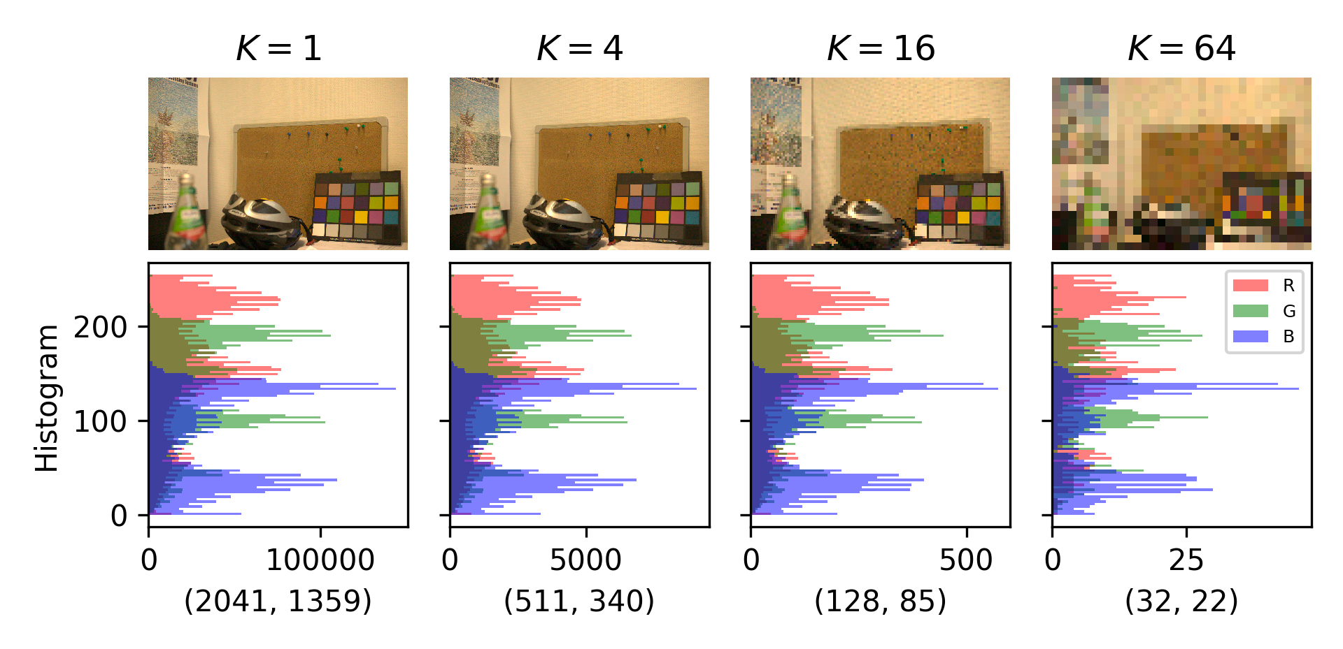
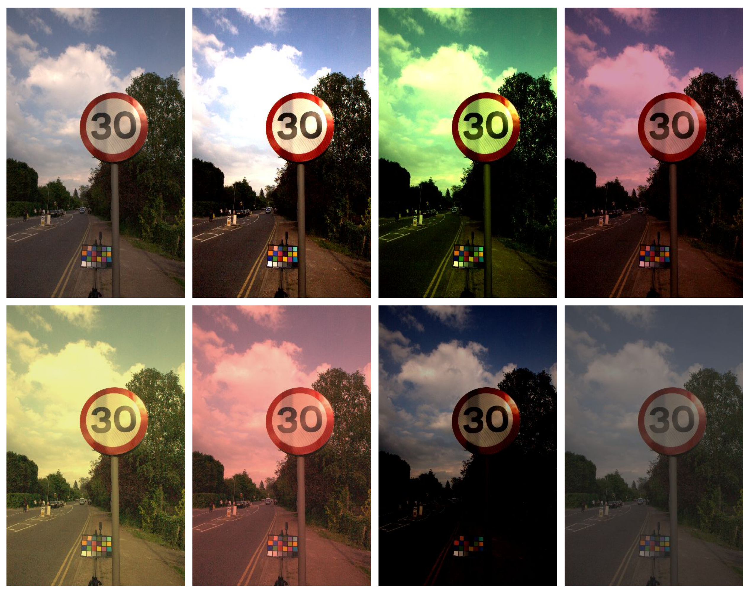
In order to benchmark the performance of all the correction methods, we implemented different metrics. First, a within-distance (\(\overline{\Delta_{RGB}}_{,within}\)) as the mean distance of all and only the colors in the ColorChecker to their expected corrected values [15]:
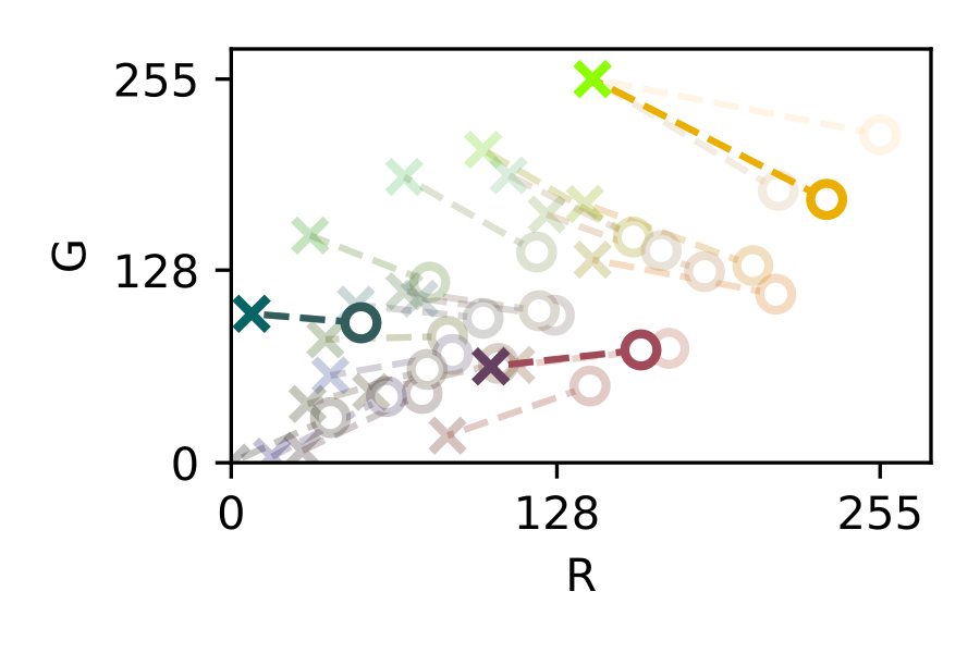
\[\overline{\Delta_{RGB}}_{,within} = \frac{\sum_{l=1}^{L} \Delta_{RGB} (\mathbf{s'}_l, \mathbf{c'}_l) }{L} \label{eq:within_distance}\]
where \(\mathbf{s'}_l\) is the corrected version of a certain ColorChecker captured color \(\mathbf{s}_l\), which has a ground-truth reference value of \(\mathbf{c'}_l\), and \(L\) is the number of reference colors in the ColorChecker (in our case \(L = 24\)). Alongside with this metric, a criterion was defined to detect failed corrections. We consider failed corrections those which failed to reduce the within-distance between the colors of the ColorChecker after the correction. Then, by comparing the \(\overline{\Delta_{RGB}}_{,within}\) of the corrected image and the image without correction (NONE):
\[\overline{\Delta_{RGB}}_{,within} - \overline{\Delta_{RGB}}_{,within,NONE} > 0 \ . \label{eq:within_comparisom}\]
Second, we defined a pairwise-distance set (\(\mathbf{\Delta_{RGB}}_{,pairwise}\)) as the set of the distances between all the colors in a ColorChecker in the same image:
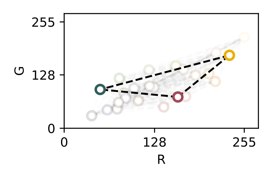
\[\mathbf{\Delta_{RGB}}_{,pairwise} = \left\{ \Delta_{RGB} (\mathbf{c}'_l, \mathbf{c}'_m ) \ : \ l,m = 1, \dots, L \right\} \label{eq:pairwise_distance}\]
where \(\mathbf{c'}_l\) and \(\mathbf{c'}_m\) are colors of the ColorChecker in a given image. Also, we implemented another criterion to detect ill-conditioned corrections. Ill-conditioned corrections are those failed corrections in which colors have also collapsed into extreme RGB values (see [fig:corner_case_tps0]). By using the minimum pairwise-distance for a given color corrected image:
\[min \left( \mathbf{\Delta_{RGB}}_{,pairwise} \right) < \updelta \ , \label{eq:pairwise_comparison}\]
where \(\updelta\) is a constant threshold which tends to zero. Note that somehow we were measuring here the opposite to the first criterion: we expected erroneous corrected colors to be pushed away from the original colors [eq:within_comparisom]. However, sometimes they also got shrunk into the borders of the RGB cube [eq:pairwise_comparison], causing two or more colors to saturate into the same color. Also, notice that we did not define a mean pairwise-distance, \(\overline{\Delta_{RGB}}_{,pairwise}\), as it was useless to define a criterion around a variable which presented huge dispersion in ill-conditioned scenarios (e.g. colors pairs were at the same time close and far, grouped by clusters).
Third, we defined an inter-distance (\(\overline{\Delta_{RGB}}_{,inter}\)) as the color distance between all the other colors in the corrected images with respect to their values in the ground-truth images (measured as the mean RGB distance of all the colors in the image but subtracting first the ColorChecker area as proposed by Hemrit et al. [147]):
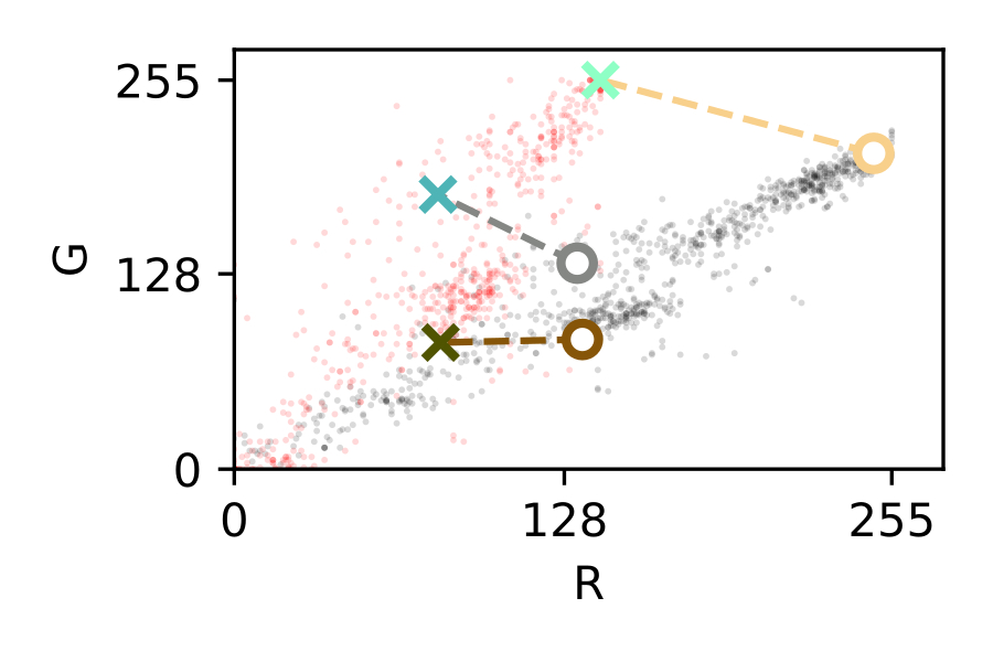
\[\overline{\Delta_{RGB}}_{,inter} = \frac{\sum_{m=1}^{M} \Delta_{RGB} (\mathbf{s'}_m, \mathbf{c'}_m) }{M} \label{eq:inter_distance}\]
where \(M\) is the total amount of pixels in the image other than those of the ColorChecker. This definition particularized the proposal of Menesatti et al., where in order to compute the \(\overline{\Delta_{RGB}}_{,inter}\), they used all the colors of another color chart instead of the actual image. Specifically, Menesatti et al. used the GretagMacbeth ColorChecker SG with 140 color patches [15].
Finally, to compare the computational performance of the methods, we measured the execution time (\(\mathcal{T}\)) to compute each corrected image, \(\mathcal{T}\) was also measured for images with different sizes to study its scaling with the amount of pixels in an image in all corrections [148].
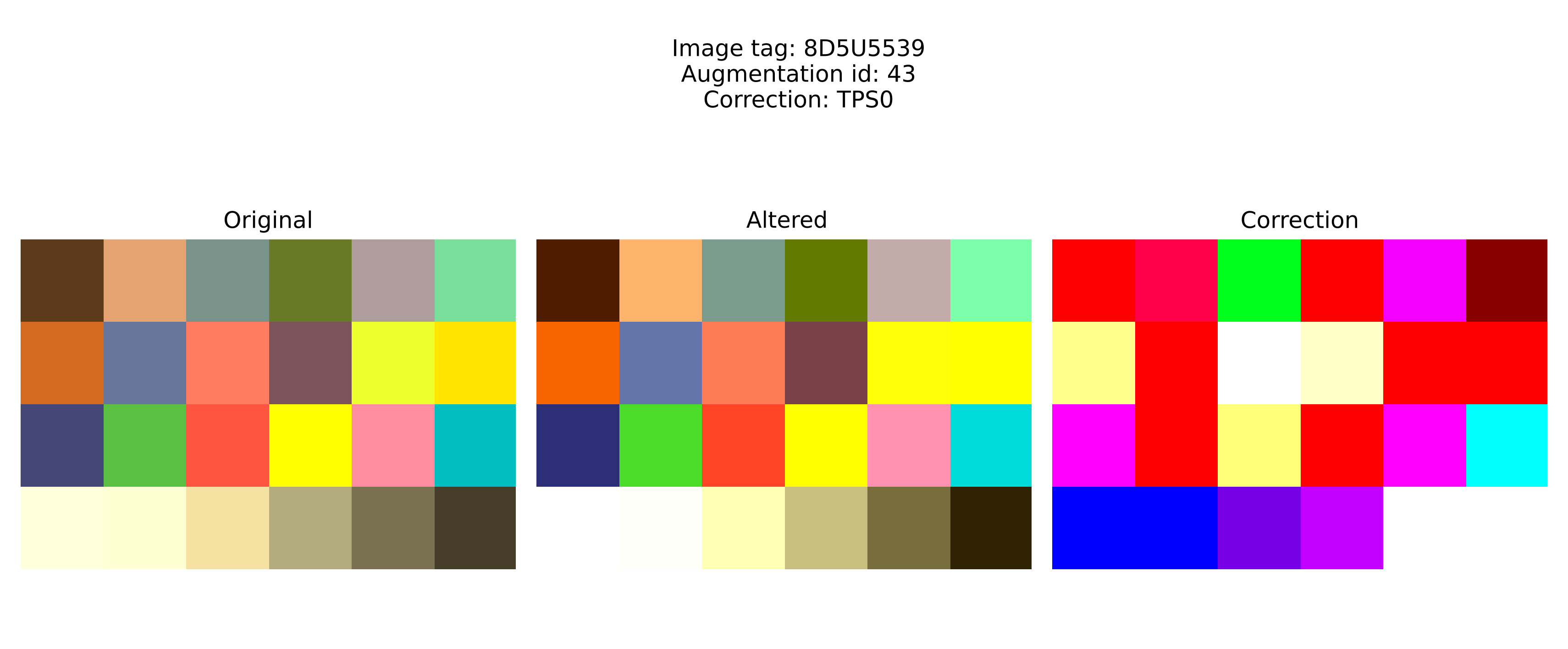
Let us start with the results of the detection of failed corrections for each color correction proposed. Here we used the defined criteria for \(\overline{\Delta_{RGB}}_{,within}\) ([eq:within_comparisom]) and \(\mathbf{\Delta_{RGB}}_{,pairwise}\) ([eq:pairwise_comparison]) to discover failed and ill-conditioned corrections (see [fig:corner_case_tps0]).
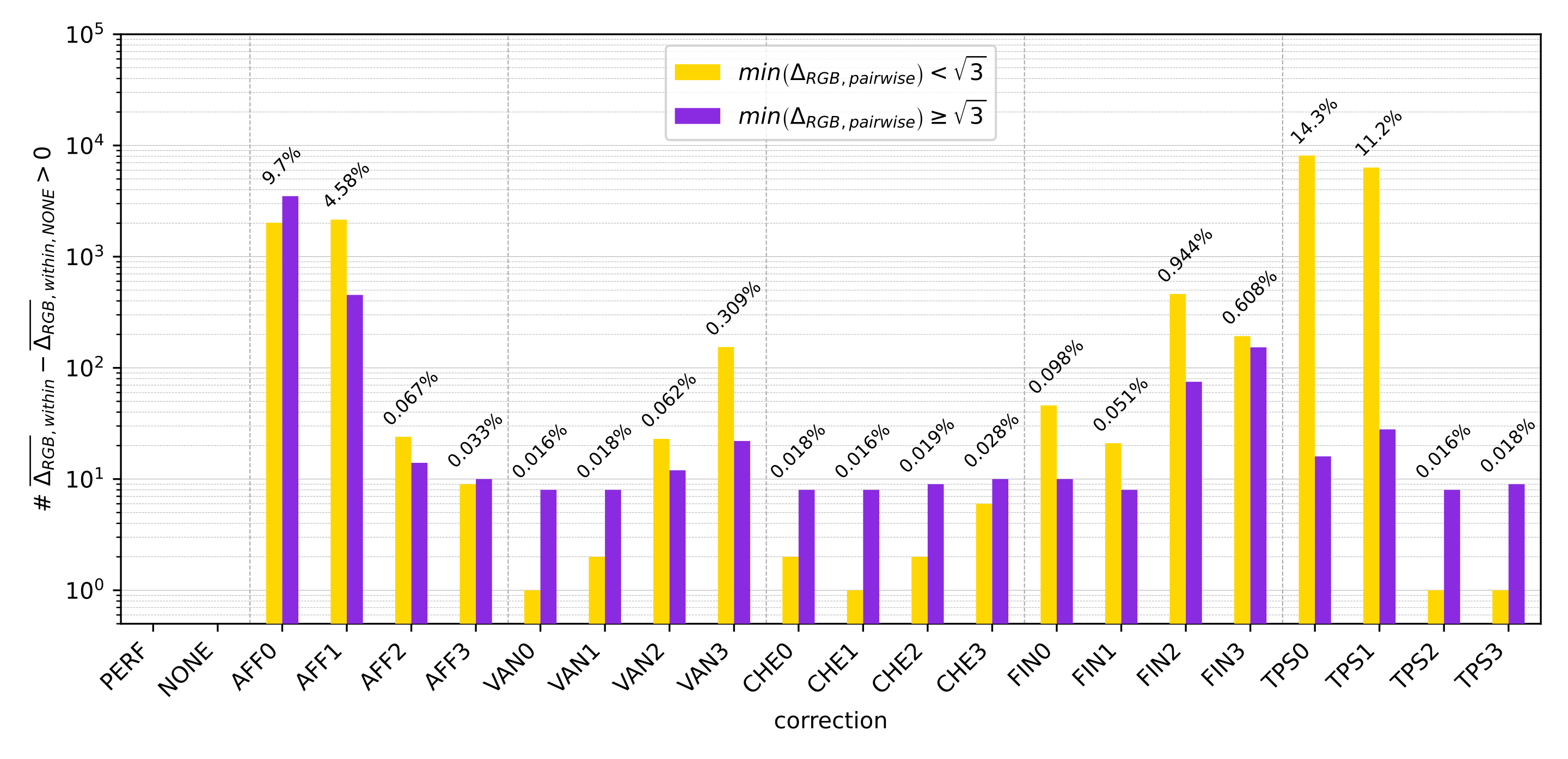
First, we subtracted the \(\overline{\Delta_{RGB}}_{,within}\) measures to the other \(\overline{\Delta_{RGB}}_{,within}\) and compared this quantity with \(\mathrm{0}\), following [eq:within_comparisom]. Those cases where this criterion was greater than \(\mathrm{0}\) were counted as failed corrections.
Second, for those corrections marked as failed, the \(\mathbf{\Delta_{RGB}}_{,pairwise}\) criteria ([eq:pairwise_comparison]) was applied to discovery ill-correction scenarios (such as [fig:corner_case_tps0]) in between failed corrections. The \(\mathbf{\Delta_{RGB}}_{,pairwise}\) criteria were implemented using a \(\updelta = \sqrt{3}\), due to the fact this is the \({\Delta_{RGB}}_{,pairwise}\) of two colors that dist one digit from each other in each channel (i.e. (0, 0, 0) and (1, 1, 1) for colors in the \(\mathbb{N}_{[0,255]}^3\) space).
Finally, we also computed the relative % of failed color corrections referenced to the total of color corrections performed. This figure is relevant as we removed these cases from further analysis.
[fig:corner_cases_count] showed how resilient the studied color correction methods are to fail, let us see how well each group of correction has scored here:
AFF: AFF0 and AFF1 scored poor results, \(\mathrm{9.7\%}\) and \(\mathrm{4.58\%}\) of failed corrections, respectively. In contrast, AFF2 and AFF3 scored almost no failure. This responds to the fact that AFF2 and AFF3 were using all the available references, instead of one or two.
Also, AFF1 reduces to a half the failed corrections from AFF0, as AFF3 reduces the AFF1 ones, as they are the same corrections but incorporating the translation component ([tab:correctionssummary]).
VAN: all four corrections scored less than a \(\mathrm{1}\)% of failed corrected images. Notice here that the degree of the polynomial expansion (from 2 to 5, VAN0 to VAN3) correlates with the amount of failed corrections. Specially for those scenarios that present ill-conditioned results, where \(min \left( \mathbf{\Delta_{RGB}}_{,pairwise} \right) < \sqrt{3}\).
CHE: all four corrections scored less than \(\mathrm{1}\)% of failed corrected images. Results were very similar to VAN corrections. The correlation between the degree of the polynomial expansion ([tab:correctionssummary]) and the failed corrections was also observed here (AFF1 to AFF3).
FIN: all four correction scored less than \(\mathrm{1}\)% of failed corrected images. Root-polynomial corrections (FIN1 and FIN3) showed around the half of failed corrections than their respective polynomial corrections (FIN0 and FIN2). But, all of them scored worse results than VAN0, VAN1 and all four CHE. This might be linked to the fact that FIN corrections did not implement the translation component to the expansion ([tab:correctionssummary]), as AFF0 and AFF2.
TPS: TPS1 and TPS0 scored the worst results in [fig:corner_cases_count], \(\mathrm{11.2}\)% and \(\mathrm{14.3}\)% of failed cases, respectively, with a huge presence of ill-conditioned results. In contrast, TPS2 and TPS3 scored in the top positions alongside with VAN0, VAN1, CHE0 and CHE2. It was easy to conclude that our proposition to smooth the thin-plate contributions to the color correction had succeeded in terms of fixing ill-conditioned scenarios (such as [fig:corner_case_tps0]).
Once evaluated and cleaned the failed corrections from our results, we proceeded to evaluate how the proposed color corrections scored in terms of color correction quality. In other words, we evaluated how they minimize the median value of the within-distances distributions and the inter-distances distributions. [fig:within_distances_zoom] and [fig:inter_distances_zoom].
We defined \(\overline{\Delta_{RGB}}_{,within}\) and \(\overline{\Delta_{RGB}}_{,inter}\) similar to Menesatti et al. [15], but it is also interesting to define these metrics with a percentage definition. The maximum distance in the RGB space is the distance \(\Delta_{RGB}((0, 0, 0), (255, 255, 255)) = 255 \cdot \sqrt{3}\), following [eq:rgb_distance]. Thus,
\[\Delta_{RGB} [\%] = 100 \cdot \frac{\Delta_{RGB}}{255 \cdot \sqrt{3}}\]
[fig:within_distances_zoom] and [fig:inter_distances_zoom] show the results with both definitions.
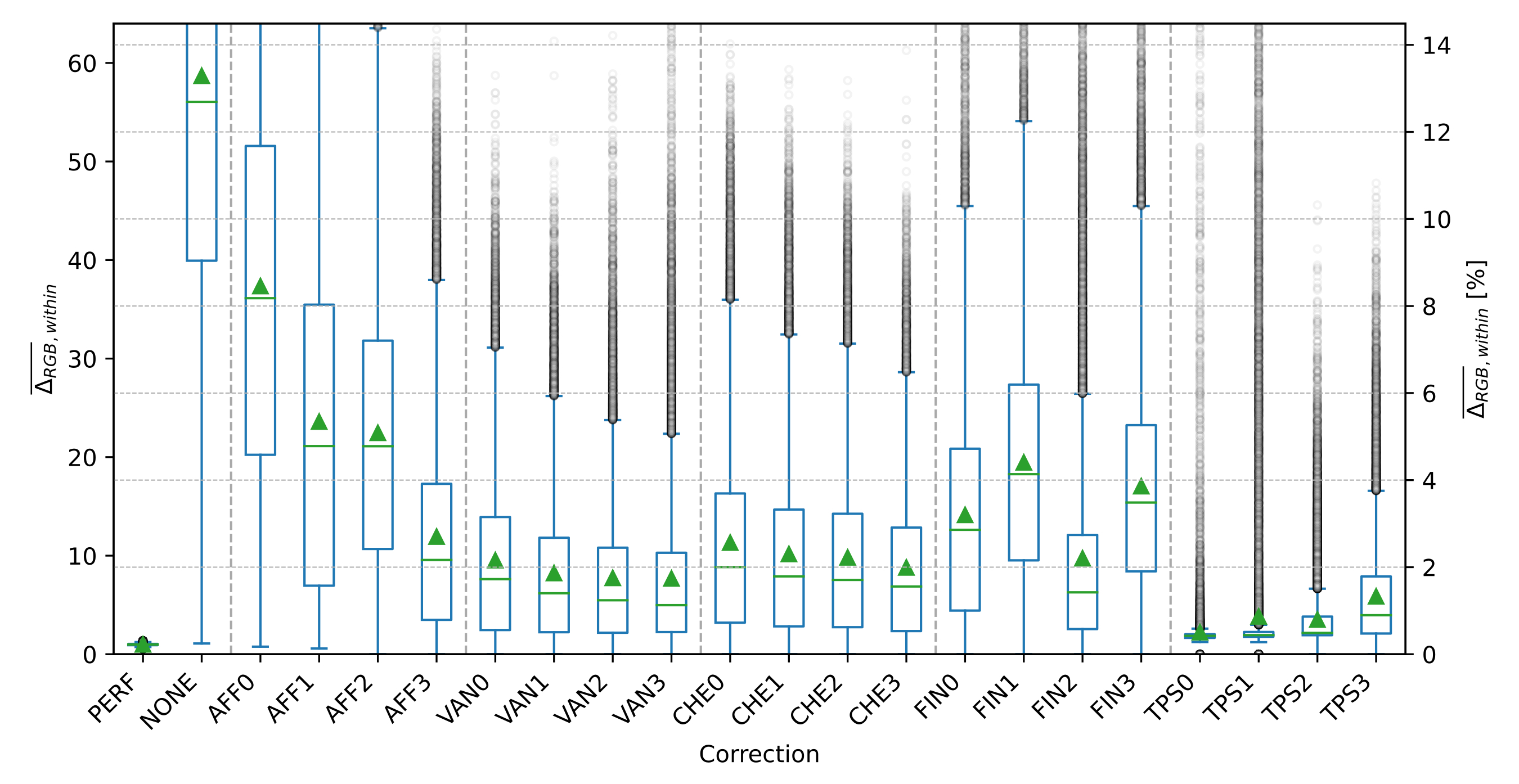
On one hand, let us see how well each group of corrections has scored in the \(\overline{\Delta_{RGB}}_{,within}\) metric (see [fig:within_distances_zoom]):
AFF: as expected AFF0, the white-balance correction, scored poorly. It was the worst correction, scoring a mean \(\overline{\Delta_{RGB}}_{,within}\) of more than \(\mathrm{8}\)%. This is due to the fact that only one color reference (white) was taken into account to compute this color correction. AFF1 and AFF2 scored a similar mean \(\overline{\Delta_{RGB}}_{,within}\) above \(\mathrm{5}\)%. AFF2, the most complete affine correction, scored the best result in this group with around a \(\mathrm{3}\)%. Also, the addition of a translation component (AFF1 and AFF3 in [tab:correctionssummary]), reduced the \(\overline{\Delta_{RGB}}_{,within}\).
VAN: all four VAN corrections scored a better mean and median \(\overline{\Delta_{RGB}}_{,within}\) than AFF3, all scoring around \(\mathrm{2}\)% or less. This was good news: here it can be seen that systematically increasing the degree of a polynomial expansion results in a better fitting of the RGB color space deformation. Despite this, results showed how this method seems to converge to a minimum median \(\overline{\Delta_{RGB}}_{,within}\) around \(\mathrm{1}\)%.
CHE: all four CHE corrections scored a better mean and median \(\overline{\Delta_{RGB}}_{,within}\) than AFF3, but they scored slightly worse results than VAN corrections (\(\mathrm{3}\)-\(\mathrm{1}\)%). This result showed that adding cross-term contributions to the polynomial expansion ([tab:correctionssummary]) did not improve the fitting of the RGB color space deformation.
FIN: surprisingly FIN corrections scored the worse results above all the polynomial corrections -VAN and CHE- (\(\mathrm{5-3\%}\)). This might be explained by the lack of translation components ([tab:correctionssummary]). Also, FIN1 and FIN3 (the root-polynomial) scored around \(\mathrm{2}\)% more \(\overline{\Delta_{RGB}}_{,within}\) than their respective polynomial corrections FIN0 and FIN2 ([tab:correctionssummary]).
TPS: all TPS corrections scored the best results for this metric. TPS0 and TPS1 scored an incredible good result of less than \(\mathrm{1}\)% of mean \(\overline{\Delta_{RGB}}_{,within}\). Here it can be seen that the outlying behavior of TPS0 and TPS1 was not fully solved before, as the mean \(\overline{\Delta_{RGB}}_{,within}\) of TPS1 is outside the distribution box. Also, TPS2 and TPS3, which approximated the TPS method to the AFF3 method scored also excellent results, better than VAN3, which is the best polynomial correction. Moreover, we checked with these results that increasing the smooth factor in the TPS formulation (TPS1 → TPS2 → TPS3), increased the \(\overline{\Delta_{RGB}}_{,within}\) as it smoothed the fitting RGB space color deformation.
On the other hand, let us see how well each group of correction has scored in the \(\overline{\Delta_{RGB}}_{,inter}\) metric (see [fig:inter_distances_zoom]):
AFF: these corrections showed somehow expected results, as they scored similar \(\overline{\Delta_{RGB}}_{,inter}\) than \(\overline{\Delta_{RGB}}_{,within}\). \(\overline{\Delta_{RGB}}_{,inter}\) increased around \(\mathrm{1-2\%}\) for all corrections, compared to \(\overline{\Delta_{RGB}}_{,within}\). AFF3 was the best of the AFF corrections, performing a mean and median inner-distance around \(\mathrm{4}\)%.
VAN: VAN0 and VAN1 presented similar results to AFF3, mean \(\overline{\Delta_{RGB}}_{,inter}\) were around \(\mathrm{4}\)%, and the distribution matched AFF3 distribution (mean, median, box and outliers). VAN2 and VAN3 presented worst results, their distributions got spread. VAN2 and VAN3 scored mean \(\overline{\Delta_{RGB}}_{,inter}\) around \(\mathrm{8}\)%. Despite the higher degree polynomial expansions systematically reduced the \(\overline{\Delta_{RGB}}_{,within}\), they increased the \(\overline{\Delta_{RGB}}_{,inter}\).
CHE: all four corrections scored similar results to AFF3, matching the AFF3 distribution (mean, median, box and outliers). Thus, performing a mean and median inner-distance around \(\mathrm{4}\)%.
FIN: all four corrections scored the worst results. FIN0 and FIN1 scored similar to AFF1 and AFF2. FIN3 showed the worst correction of the overall data, above AFF0 and VAN3, with a median \(\overline{\Delta_{RGB}}_{,within}\) of almost \(\mathrm{10\%}\), and a mean of almost \(\mathrm{8}\)%. Once again, it was observed that root-polynomial presents worst results than their respective polynomial correction.
TPS: all four correction scored the best results also for this metric. The effect of smoothing or not the TPS correction was smaller in this metric. All four corrections scored median and mean \(\overline{\Delta_{RGB}}_{,inter}\) around \(\mathrm{2\%}\).
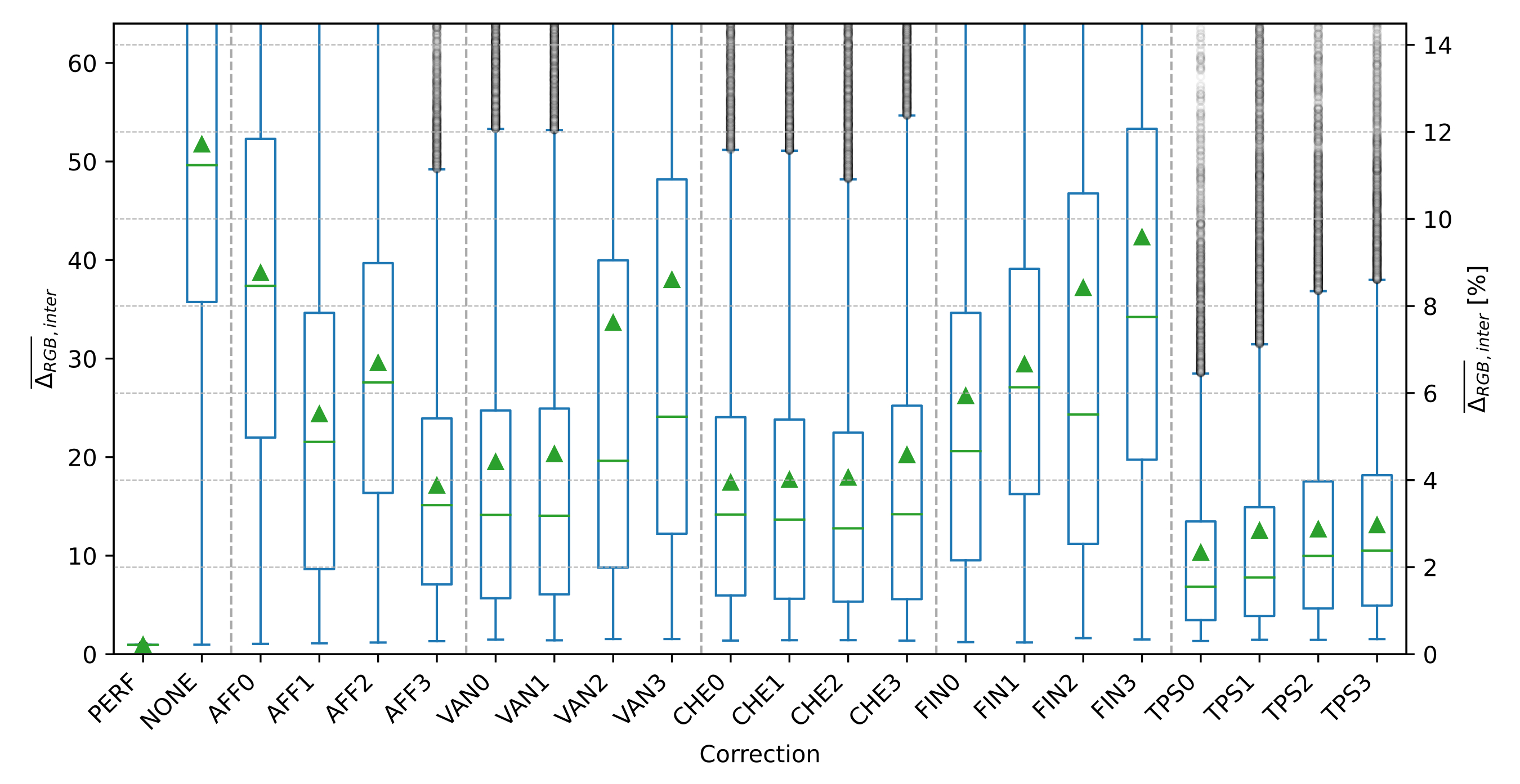
All in all, TPS corrections proved to provide the best solution to color correct images in our dataset. The original Menesatti et al. [15] proposal (TPS0) worked slightly better than our first proposal of using the recommended RBF for 3D spaces (TPS1). The smoothed TPS proposals (TPS2 and TPS3) scored the subsequent best results for both metrics, \(\overline{\Delta_{RGB}}_{,within}\) and \(\overline{\Delta_{RGB}}_{,inter}\). VAN3 proved to be a good competitor in the within-distance metric, in contrast it had one of the poor results in the \(\overline{\Delta_{RGB}}_{,inter}\) metric. AFF3, VAN0, VAN1 and all CHE methods proved to be good competitors in the \(\overline{\Delta_{RGB}}_{,inter}\) metric, that is an interesting result as it opens the possibility to have fall-back methods if the TPS fails.
Let us see how the proposed color correction methods scored in terms of execution time for each image corrected. As our dataset has images from two cameras, with different sizes, we decided to focus only in one camera to ensure results were not affected by the disparity in size. We chose to work with the larger subset of images: the Canon EOS 5D with 483 images. These images have \(549 \times 365 \ \textrm{pixels} = 200385 \ \textrm{pixels} \approx 0.2 \ \textrm{Mpx}\) (see [tab:ccdatasetdownsampling]), as we down-sampled them (\(K = 4\)) to speed up the global computation time of our pipeline (see [fig:ccdatasetpipeline]).
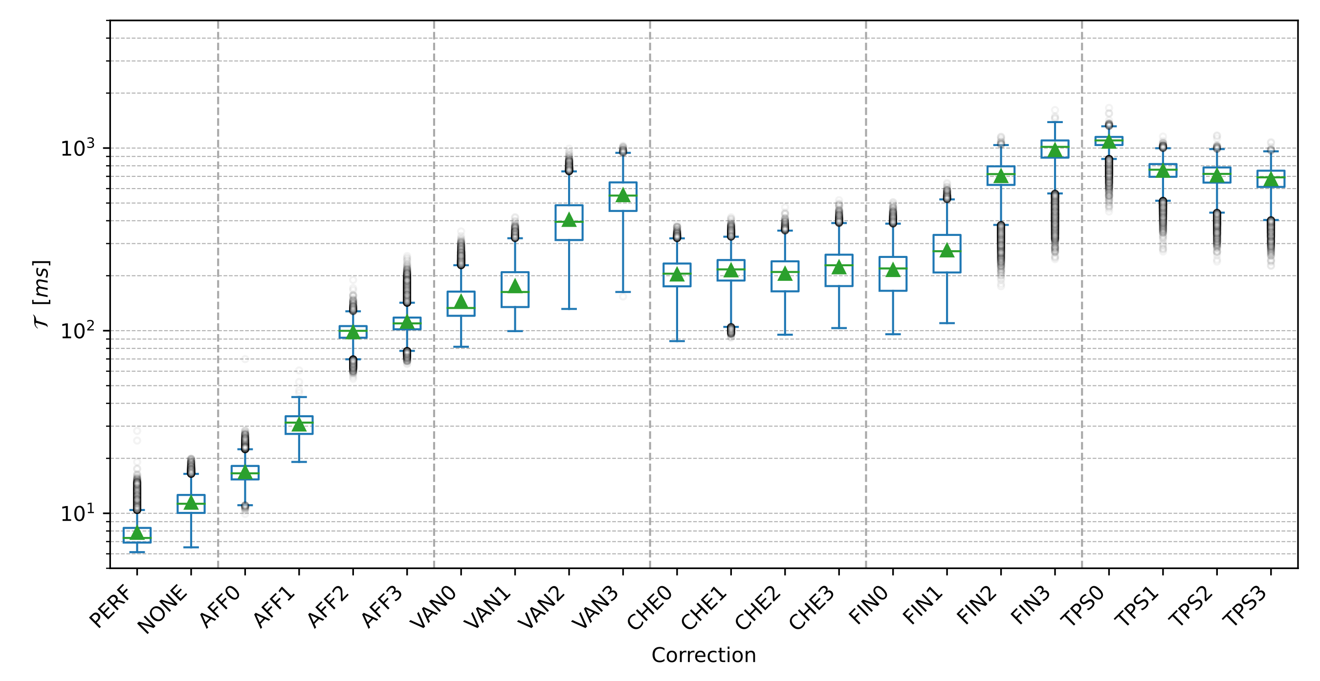
[fig:exec_time] shows the results of the measured execution times. PERF execution time represents the minimal time to compute our pipeline, as the PERF method also went all the way computing the same pipeline, it just returns the perfect expected image in 8-bit representation. NONE did the same but returning the image without applying any correction, note that this is slightly a slow process, as we are returning a different image for each augmentation. Let us see how the other methods scored in this benchmark:
AFF: all four corrections scored the best results in the benchmark, as expected, as they are the simpler corrections regarding implementation. AFF0 and AFF1 scored a mean \(\mathcal{T}\) per image around \(\mathrm{20-30}\) ms. AFF2 and AFF3 scored around \(\mathrm{100}\) ms.
VAN: all four corrections were slower than AFF3, from a \(\mathrm{100}\) ms to \(\mathrm{600}\) ms. As AFF3 is a polynomial correction of order 1, and the subsequent corrections are VAN0 to VAN3, with degrees \(\mathrm{2}\) to \(\mathrm{5}\), respectively, we can observe \(\mathcal{T}\) increases with the degree.
CHE: all four corrections scored similar results to VAN1, with a mean \(\mathcal{T}\) per image around \(\mathrm{200}\) ms. Being around \(\mathrm{10}\) times slower than AFF0 and \(\mathrm{2}\) times slower than AFF2-AFF3.
FIN: FIN0 scored very similar to the above-mentioned CHE methods. Despite this good result, the other FIN displayed slow mean \(\mathcal{T}\) per image. FIN3 takes around \(\mathrm{1000}\) ms to compute an image. In FIN methods again, adding superior degrees to the polynomial expansion adds computational time to the correction. Also, adding complex operation to the pipeline, such as computing a root square, also affects the computational cost of the solution.
TPS: TPS0 scored very similar to FIN3, and in fact scored above the mean \(\mathrm{1000}\) ms timestamp, achieving the worst score for this metric. This makes sense, as TP0 is the original TPS method, which implied the use of a more complex function (see [tab:correctionssummary]). Our proposal TPS1 reduced this computation time around 800 ms. Also, adding smooth to the TPS method seems to reduce slightly its mean \(\mathcal{T}\), arriving down to \(\mathrm{700}\) ms at TPS3. TPS3 is around \(\mathrm{25}\) times slower than AFF1 and \(\mathrm{8}\) times slower than AFF3.
All in all, results for AFF, VAN, CHE and FIN showed that increasing the degree of the polynomial expansion, increased the mean \(\mathcal{T}\) for each image. AFF corrections achieved the top scores as they are computationally simple. And, TPS scored poorly in this benchmark, as expected [148]. Also, the scores for VAN2, VAN3, FIN2 and FIN3 were also poor. We accomplished to improve slightly the TPS computational performance by introducing a change in the RBF and the smooth parameter.
Finally, as we computed the above-mentioned results using thumbnail images (\(K=4\), \(\mathrm{549\times 365}\) pixels), we wanted to check the computational order of the presented methods against the size of the image.
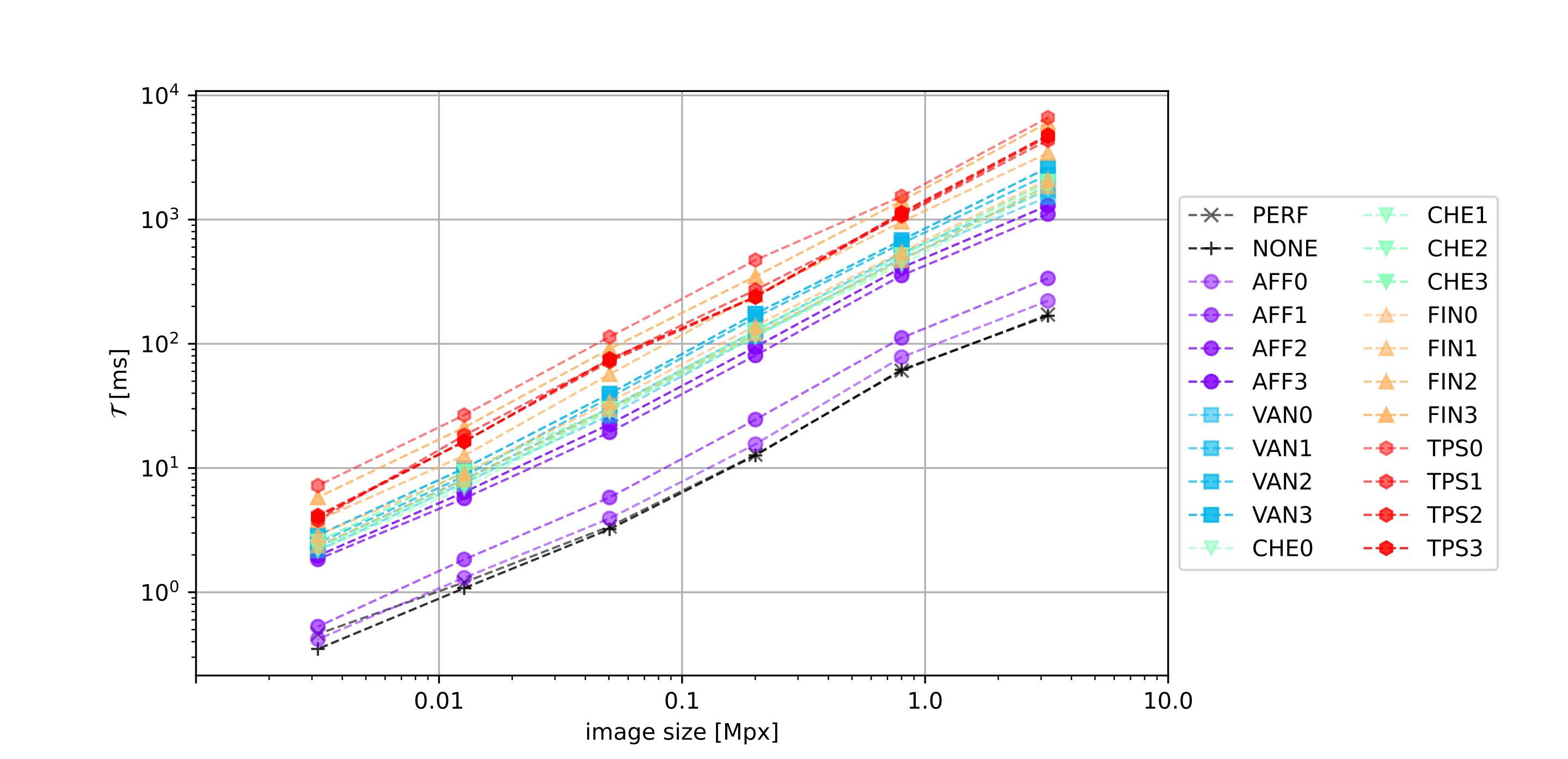
To do so, we computed a reduced dataset of images containing 10 images from the dataset and recomputed the same pipeline (see [fig:ccdatasetpipeline]) for different \(K\) down-sampling constants (see [fig:ccdatasethistogram]): \(\mathrm{1}\), \(\mathrm{2}\), \(\mathrm{4}\), \(\mathrm{8}\), \(\mathrm{16}\) and \(\mathrm{32}\). This rendered images of approximately: \(\mathrm{3.2}\), \(\mathrm{0.80}\), \(\mathrm{0.2}\), \(\mathrm{0.05}\), \(\mathrm{0.012}\) and \(\mathrm{0.003}\) megapixels, respectively.
[fig:exec_time_sizes] shows the computed results, as we can see all corrections performed with a linear computational order \(O(n)\), for the all the down-sampled versions of the images. The figure also shows the relation we found earlier between the different correction, i.e. TPS are almost two decades apart from AFF corrections. We consider these results to be useful as they could be used eventually as a design rule when designing color corrections pipelines.
In this chapter, we improved the work done by Menesatti et al. [15]. We successfully reproduced their findings about the TPS3D method for color correction to achieve image consistency in datasets. It can be shown that our results match theirs not only qualitatively but also quantitatively. For this purpose, [tab:resultssummary] shows a summary of the above-presented results for future comparison.
Also, we extended the study to other state-of-the-art methods, Gong et al. [44], Cheung et al. [27] and Finlayson et al. [28], that can be found in standard libraries [153]. The TPS3D proved to be the best correction color method among the other in terms of color correction quality, both in \(\overline{\Delta_{RGB}}_{,within}\) and \(\overline{\Delta_{RGB}}_{,inter}\) metrics. Despite this, TPS3D is a heavy implementation compared to simpler methods such as AFF color corrections, resulting in \(\mathcal{T}\) per image \(\mathrm{20}\) to \(\mathrm{100}\) times higher.
Moreover, we proposed 2 criteria to detect failed corrections using the \(\overline{\Delta_{RGB}}_{,within}\) and \(\mathbf{\Delta_{RGB}}_{,pairwise}\) metrics. These criteria discovered failed corrections over the dataset that heavily affected TPS3D. Our proposal to approximate the TPS3D formulation by a smoothing factor proved the right way to systemically remove those ill-conditioned scenarios.
Furthermore, we compared different RBF into the TPS3D formulation. This did not mean a significant improvement in the color correction, although we did find that our proposed RBF would improve by a 30% the results regarding the \(\mathcal{T}\) per image.
Finally, we demonstrated that \(\mathcal{T}\) increases linearly with the image size for all the compared color corrections, enabling to take into account this variable when designing future color correction pipelines.
Regarding future work to improve this color correction framework, let us highlight some alternatives.
First, the systematic increase of color references should lead to a systematic improvement. This was not explored in the presented work in the chapter. As explained we preferred to use an established dataset which contained only images with the original ColorChecker with 24 color patches [13].
Thus, if creating a new dataset, one could add to the images modern color charts from X-Rite which include up to 140 colors, as other authors did [15], [154], [155]. Or, one could use directly our proposal of [ch:5] to encode the same 140 color references in our proposed back-compatible QR Code.
We deepen into this idea of using our machine-readable patterns in [ch:7], where we used a Color QR Code to embed 125 colors of the RGB cube and use those colors with the above-presented color correction framework.
Second, we proposed this color correction framework as a solution to a general-purpose image consistency scenario. Often, colorimetric problems present themselves as a more reduced problem, i.e. we only need to seek for color correction in a certain subset of colors. If this is the case, instead of increasing the amount of correction colors we could reduce the colors to perform the color correction.
When doing so, we ought to select the color references which are near our data points, or at least they are the most representative version of our data within our correction colors. If not, the mapping will be poor in some parts of the data, as Donato et al. pointed out when discussing different approximation techniques for TPS mappings [125].
Third, there exist several authors that have explored different RBF that could be placed in the kernel definition of the TPS3D method, here we only discussed between two RBF which were solutions for 2D and 3D for the thin-plate spline solution. Theoretically, any RBF could be used [144], and even more modern smooth bump functions [156], [157] as well.
| Correction | #1 | #2 | #3 | #4 | #5 | #6 | #7 | ||||
| - | - | \(\upmu\) | \(\upsigma\) | \(\tilde{\upmu}\) | \(\upmu\) | \(\upmu\) | \(\upsigma\) | \(\tilde{\upmu}\) | \(\upmu\) | \(\upmu\) | |
| PERF | 0 | 0 | 0.99 | 0.12 | 0.99 | 0.223 | 0.945 | 0.019 | 0.949 | 0.214 | 8 |
| NONE | 0 | 0 | 59 | 27 | 56 | 13 | 52 | 23 | 50 | 12 | 11 |
| AFF0 | 5519 | 2018 | 37 | 21 | 36 | 8 | 39 | 22 | 37 | 9 | 17 |
| AFF1 | 2605 | 2152 | 24 | 18 | 21 | 5 | 24 | 19 | 22 | 6 | 30 |
| AFF2 | 38 | 24 | 22 | 14 | 21 | 5.1 | 30 | 17 | 28 | 7 | 96 |
| AFF3 | 19 | 9 | 12 | 10 | 10 | 2.7 | 17 | 12 | 15 | 3.9 | 110 |
| VAN0 | 9 | 1 | 10 | 8 | 8 | 2.2 | 20 | 22 | 14 | 4 | 142 |
| VAN1 | 10 | 2 | 8 | 7 | 6 | 1.9 | 20 | 23 | 14 | 5 | 172 |
| VAN2 | 35 | 23 | 8 | 7 | 5 | 1.8 | 30 | 40 | 20 | 8 | 397 |
| VAN3 | 176 | 154 | 8 | 8 | 5 | 1.7 | 40 | 40 | 20 | 9 | 542 |
| CHE0 | 10 | 2 | 11 | 9 | 9 | 2.6 | 17 | 15 | 14 | 3.9 | 199 |
| CHE1 | 9 | 1 | 10 | 9 | 8 | 2.3 | 18 | 18 | 14 | 4 | 210 |
| CHE2 | 11 | 2 | 10 | 8 | 8 | 2.2 | 18 | 22 | 13 | 4 | 202 |
| CHE3 | 16 | 6 | 9 | 7 | 7 | 2.0 | 20 | 25 | 14 | 5 | 219 |
| FIN0 | 56 | 46 | 14 | 11 | 13 | 3.2 | 26 | 24 | 21 | 6 | 212 |
| FIN1 | 29 | 21 | 19 | 12 | 18 | 4.4 | 29 | 18 | 27 | 7 | 271 |
| FIN2 | 537 | 462 | 10 | 11 | 6 | 2.2 | 40 | 40 | 20 | 8 | 691 |
| FIN3 | 346 | 193 | 17 | 11 | 15 | 3.9 | 42 | 34 | 34 | 10 | 958 |
| TPS0 | 8133 | 8117 | 2 | 7 | 2 | 0.5 | 10 | 13 | 7 | 2.3 | 1067 |
| TPS1 | 6359 | 6331 | 4 | 10 | 2 | 0.9 | 13 | 16 | 8 | 3 | 738 |
| TPS2 | 9 | 1 | 3.5 | 3.3 | 2.2 | 0.8 | 13 | 11 | 10 | 2.9 | 697 |
| TPS3 | 10 | 1 | 6 | 5 | 4 | 1.3 | 13 | 11 | 11 | 3.0 | 665 |
Table headers:
| #1: | \(\overline{\Delta_{RGB}}_{,within} - \overline{\Delta_{RGB}}_{,within,NONE} > 0\) | [u.] |
| #2: | \(min \left( \mathbf{\Delta_{RGB}}_{,pairwise} \right) < \sqrt{3}\) | [-] |
| #3: | \(\overline{\Delta_{RGB}}_{,within}\) | [-] |
| #4: | \(\overline{\Delta_{RGB}}_{,within}\) | [%] |
| #5: | \(\overline{\Delta_{RGB}}_{,inter}\) | [-] |
| #6: | \(\overline{\Delta_{RGB}}_{,inter}\) | [%] |
| #7: | \(\mathcal{T}\) | [ms] |
In previous chapters, we presented the need to achieve consistency in image datasets, and how this need relates to the capacity to perform quantitative color measurements over those datasets. Also, we discussed how this need is relevant in several industries. In this chapter, we are going to focus on the application of color consistency in analytical chemistry [4], specifically in environmental sensing.
Environmental sensing is a wide field of research. For example, one could tackle the problem using electronic sensors [158]. Or, one could use colorimetric indicators. Colorimetric indicators are present in our daily life as humidity [39], temperature [40] or gas sensors [41], [42].
Usually, colorimetric indicators feature chemical reactions which act as a sensor or dosimeter for a certain substance or physical magnitude. A change on these magnitudes is then translated into a change in the color of the chemical solution, e.g. a pH change that induces a change in the chemical structure of a molecule which renders the color change (see [fig:engel_chem]).
Moreover, colorimetric indicators are inexpensive and disposable, and simple to fabricate, for example, printing them on top of a cellulose paper [31].
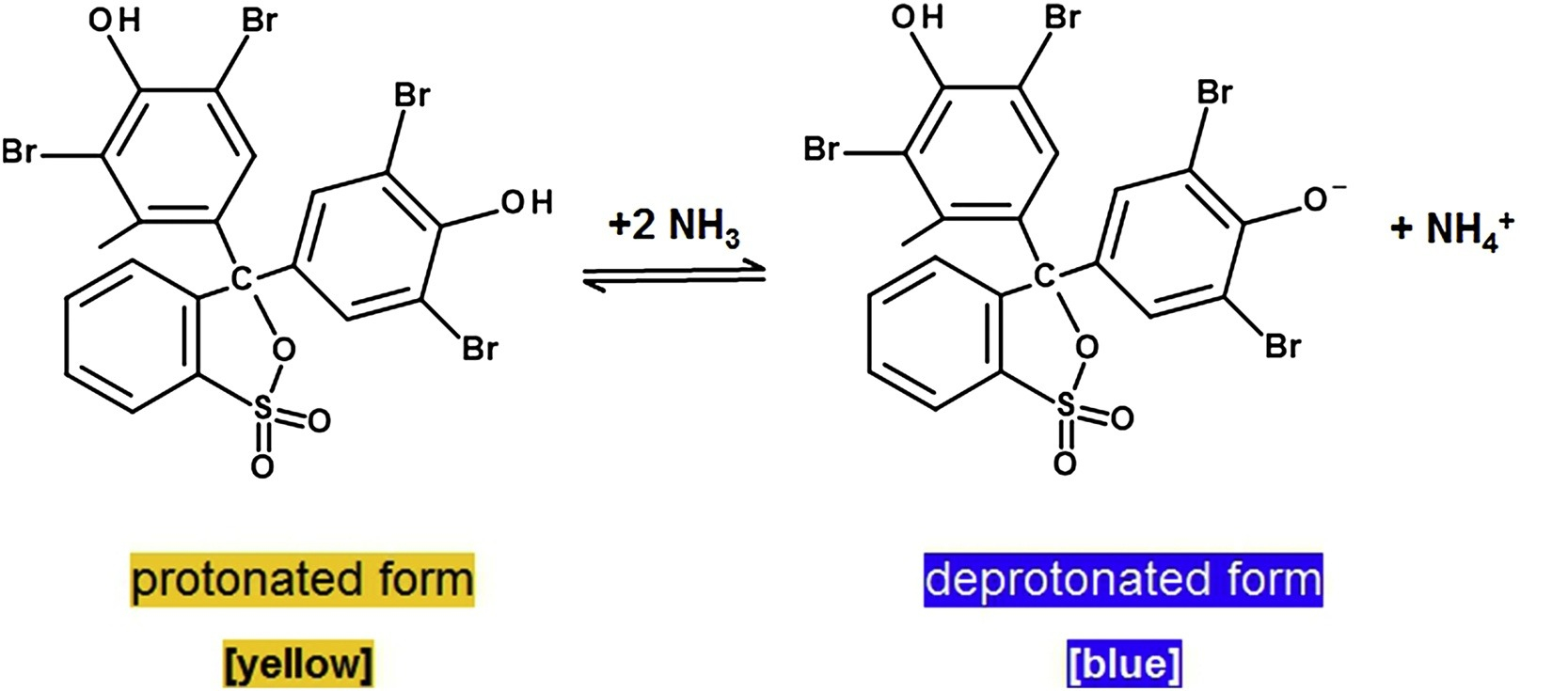
In 2017, within a related research project, we presented a solution to detect nitrogen dioxide (\(NO_2\)) in the environment using a colorimetric indicator. In that work, the colorimetric indicators were prepared soaking sterilized absorbent cellulose into the reactive ink. The results successfully concluded that it was possible to measure air concentrations of \(NO_2\) from \(\mathrm{1}\) ppm to \(\mathrm{300}\) ppm in air using a colorimetric indicator [3], [159] (see [fig:fabrega_no2]).
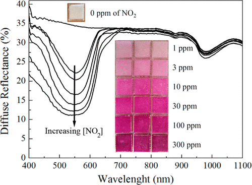
Later that year, we also presented a solution to detect ammonia (\(NH_3\)) in the environment with colorimetric indicators. In that case, the colorimetric indicators were created dip-coating a glass substrate in a solution containing the reactive ink (see [fig:nh3_dip_coating]). Results showed that it was possible to measure concentrations of \(NH_3\) from \(\mathrm{10}\) to \(\mathrm{100}\) ppm in air [160].
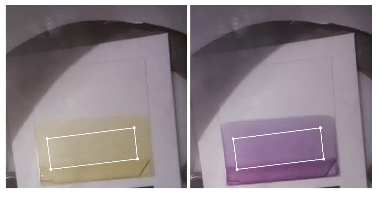
In both works, we did not measure the color with digital cameras. On one hand, the \(NO_2\) sensor was enclosed in a setup with a fixed one-pixel RGB sensor (TCS3200) and four LED acting as a light source. This research line was used in parallel as an alternative, a reference to understand color changes by enclosing colorimetric sensors in controlled compact and cost-effective fixed setups [45], [161], [162].
On the other hand, the \(NH_3\) sensor was studied using standard spectrophotometry and the sRGB color was computed from the measured spectra (see [fig:human_vision_nh3]). The work presented here is the continuation of our contribution to solve this problem using digital cameras without the need to enclose the sensor in a setup [29], [30], [163].
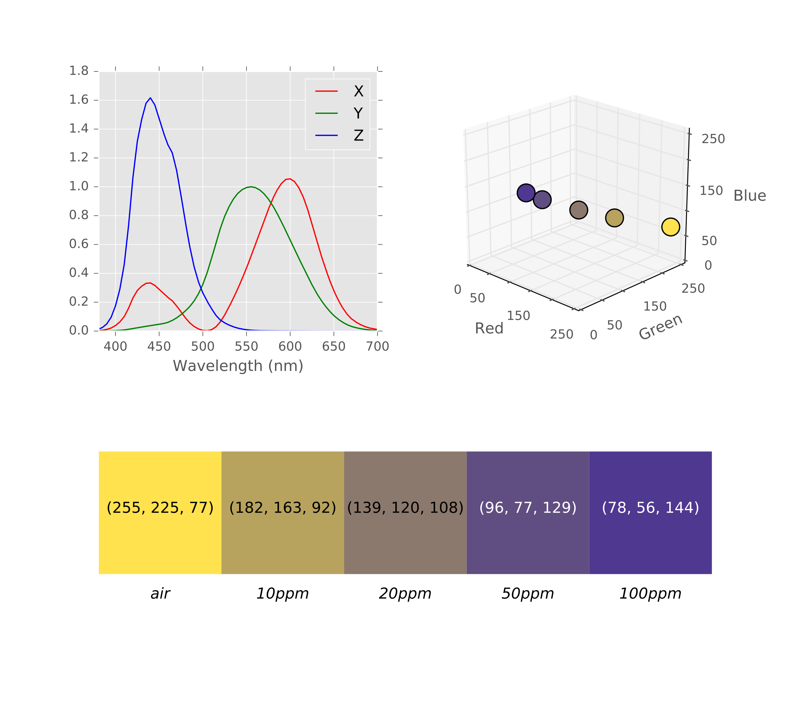
In this chapter, we present the different partial approaches to combine colorimetric indicators that led to the thesis proposal of Color QR Codes. The partial solutions were applied to different target gases, such as ammonia, (\(NH_3\)), hydrogen sulfide (\(H_2S\)), etc.
Finally, we present here a carbon dioxide (\(CO_2\)) sensor featured in a Color QR Code. The Color QR Code enables to: extract the sensor from any surface ([ch:4]), embed inside or outside the QR Code the sensor ink ([ch:5]) alongside with color references to perform a color correction using the whole range of corrections studied ([ch:6]).
In 2018, we presented a solution [29] to automate the readout of an environmental colorimetric indicator that was developed to detect \(NH_3\) [160]. This solution preceded most of the research presented in this thesis.
The proposal was to design a machine-readable pattern resembling a QR Code, without any digital data, to allocate color references and two reserved areas to print the colorimetric ink. The whole process of design, fabrication and interrogation is described in [fig:ibenito_pipeline].
The machine-readable pattern would maintain the finder, alignment and timing patterns of QR Codes (more details in [ch:3]). [fig:ibenito_qr] shows an example of these machine-readable patterns designed to embed a \(NH_3\) sensor.
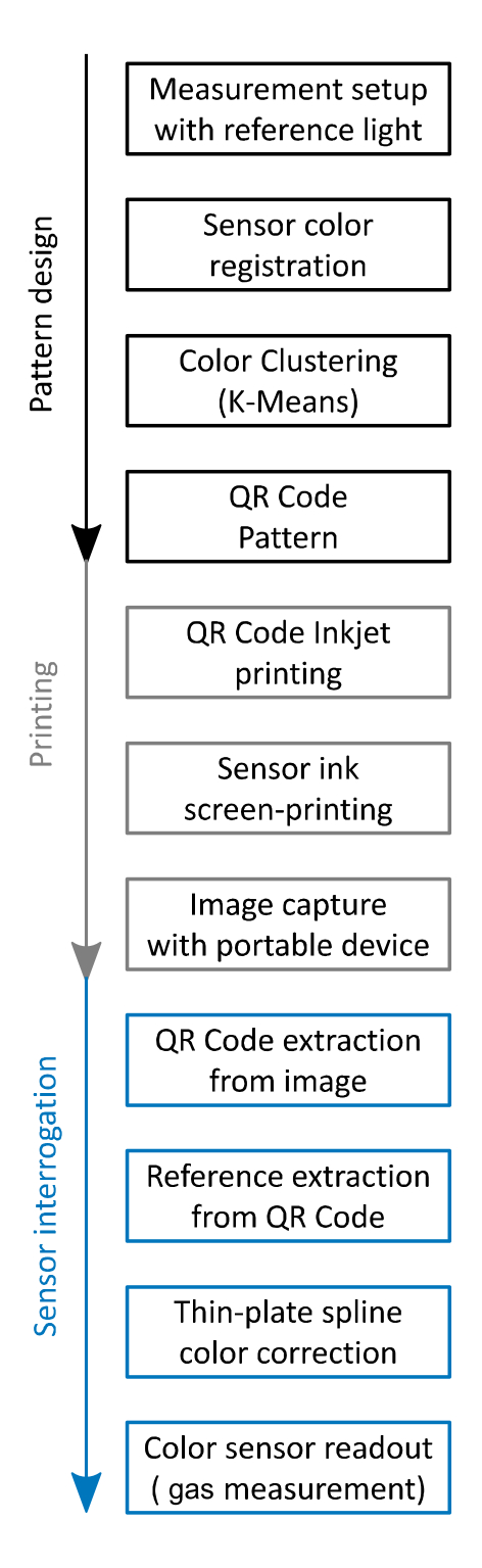
The first downside of this proposal is the way the color references are generated. These colors derived from the measures of the ink color when exposed to different amounts of the target gas – \(NH_3\) – (see [fig:nh3_sensor_registration]), and then classified into a subset of colors – e.g. 32 colors – (see [fig:nh3_color_clustering]). Later, when the machine-readable pattern was printed, the color might differ from the measured color. This is a perfect example of trying to solve the problem of color reproduction. As we discussed in previous chapters, we rather solved the image consistency problem, i.e. place more color references than only those colors from the sensor.
The second downside was the way these color references were encoded in the QR Code-like pattern. As we cleared all the digital information area, we invalidated one of our goals: to achieve a back-compatible QR Code for colorimetric applications. Also, this proposal embedded the colors in \(3 \times 3\) module blocks as we did not develop yet the proper methods to correctly perform a successful extraction in challenging surfaces without significant readout failures.
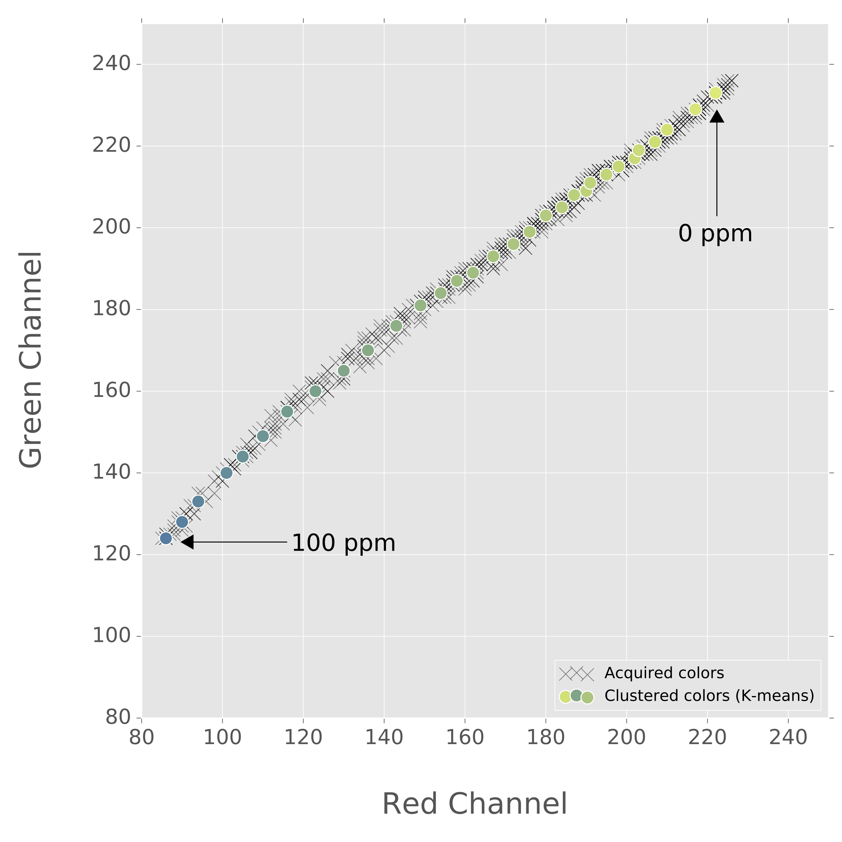
![32 clusters centers from data in [fig:nh3_sensor_registration], and color clustering regions. Data is presented as a projection into the red-green plane of the RGB space.](assets/graphics/chapters/chapter7/figures/color_clustering_kmeans.jpg)
In 2020, we introduced our improved proposal for a machine-readable pattern for colorimetric indicators [30], [163]. This approach maintained the use of a QR Code-like machine-readable pattern without digital data, only allocating the sensor ink, the color references and computer vision patterns to perform the readout.
However, as we improved our computer vision algorithms to capture QR Codes, we were able to add more complex color encoding to the pattern definition. Then, the number of embedded color references in the pattern was considerably increased, and therefore the color correction method was improved (see [fig:engel_layers]).
This proposal tackled many aspects of the sensor readout improving the former ones:
The factor form of a QR Code version \(\mathrm{7}\) was maintained, preserving the alignment pattern array to ease the readout.
An additional pattern to ease the location of the fourth corner was added.
The reference colors were embedded as \(\mathrm{1 \times 1}\) modules, this is, the same size of a QR Code module.
Two palettes of reference colors were embedded with a total of 245 colors: 125 colors from an RGB excursion, with 5 samples per channel; and 120 colors from an HSL excursion, with 6 samples for the H channel, 4 for the S channel and 5 for the L channel.
A fabrication process which involved screen-printing instead of dip-coating was used, improving the sensor reproduction.
An improved version of the TPS3D color correction which accounted for ill-conditioned scenarios and corrected them if possible with a fall-back mechanism into affine transformations was implemented in the image processing steps.
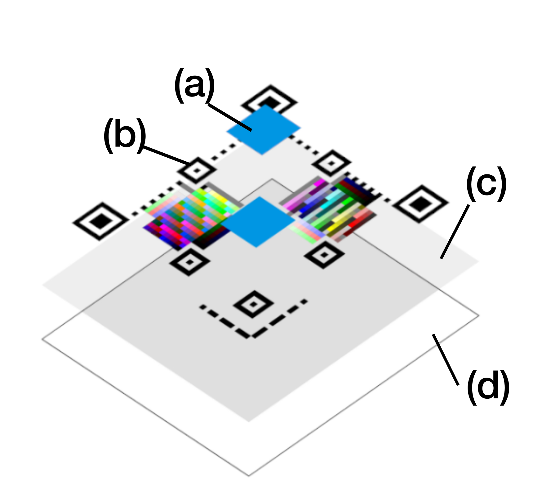
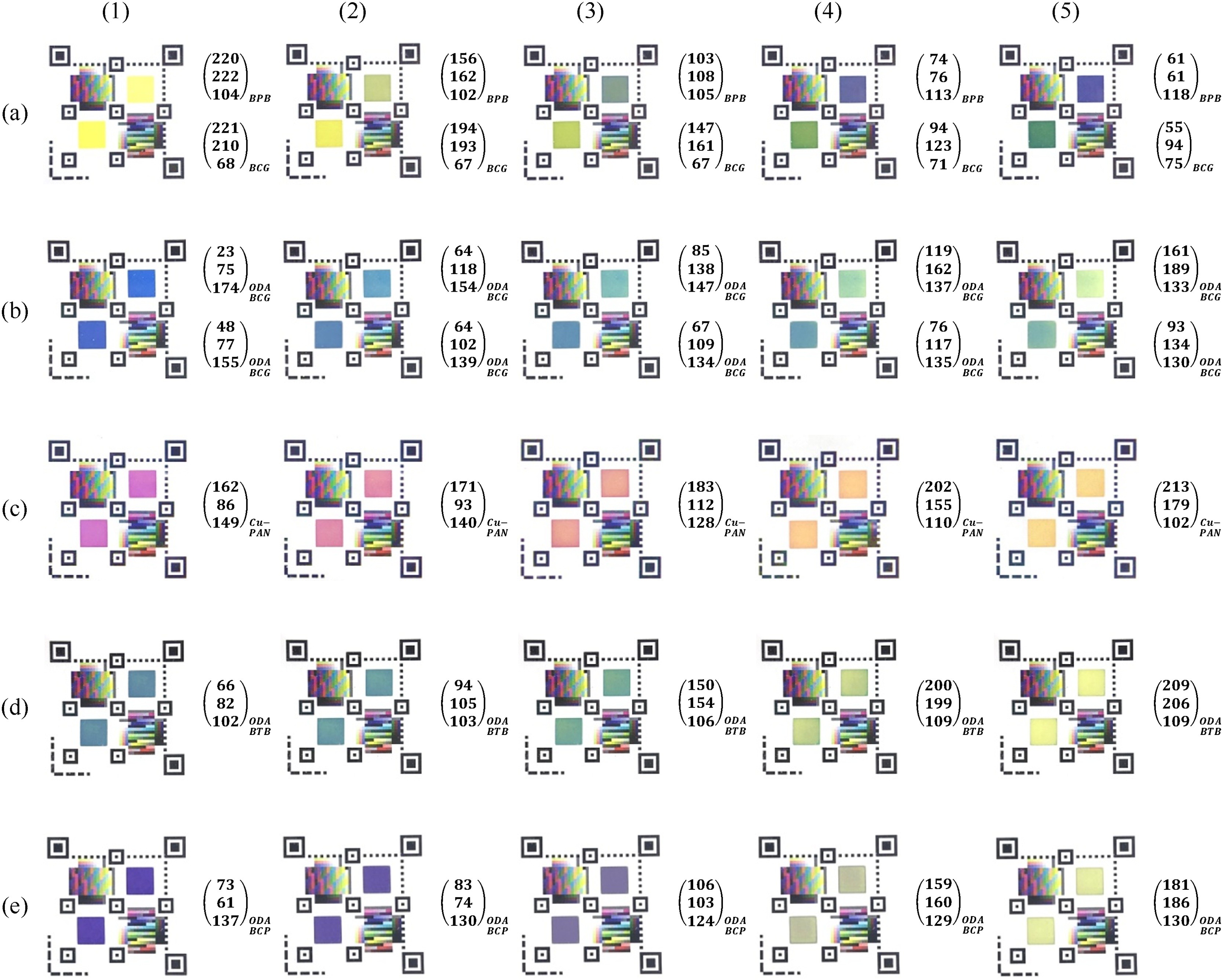
All in all, we successfully applied this proposal of machine-readable patterns which resemble a QR Code into several colorimetric indicators that targeted different environmental gases [30] (see [fig:engel_qr_table]):
\(\mathbf{NH_3}\): an ammonia sensor as a result of combining two colorimetric indicators, bromophenol blue (BPB) and bromocresol green (BCG).
\(\mathbf{H_2S}\): a hydrogen sulfide dosimeter using a copper complex of an azo dye (Cu-PAN) as colorimetric indicator.
\(\mathbf{CH_2O}\): three different dosimeters to measure formaldehyde, based on three different colorimetric indicators. Once again, based on the bromophenol blue (BPB) and bromocresol green (BCG), with the addition of an extra compound, octadecylamine (ODA), to tune the original indicator to this target gas.
Here, we present now a Color QR Code for colorimetric indicators which features fully-functional back-compatibility. This means it can be read with any commercial QR Code scanner to get a URL, or any other message (see [fig:color_qr_code]). The main specifications of these machine-readable patterns are:

They use the full standard of the QR Code. Thus:
enabling extraction techniques similar to the ones presented in [ch:4], which leads to ease the location of colorimetric elements in the same scene, placed outside the QR Code (see [fig:color_qr_code_layout].a), or inside (see [fig:color_qr_code_layout].b),
plus, they can be designed in any desired version of the QR Code standard (the current proposal uses a version 3 instead of a version 7, reducing the physical size of the sensor),
and they can encode any desired information, for example a URL with a variable ID, rendering almost infinite possibilities (see [fig:color_qr_ids])
Also, they can embed hundreds of colors, following our technique to create back-compatible QR Codes, as we detailed in [ch:5]. This implies:
they contain by default \(\mathrm{125}\) RGB colors (\(5 \times 5 \times 5\)),
\(\mathrm{100}\) of them are encoded in the DATA zone of the QR Code,
\(\mathrm{25}\) of them are encoded in the EC zone of the QR Code,
and more extra slots to allocate reactive inks, that account in the design of the QR Code as errors.
![The structure of the Color QR Code from [fig:color_qr_code]. (a) and (b) show possible sensor inks placements, (a) shows a big sensor outside the QR Code, (b) shows smaller factor forms (3 \times 2, 1 \times 1, ...) inside the QR Code. (c) Shows the color references and how they are spread in the QR Code areas. Finally, (d) shows the whole layout of the sensor with the Color QR Code.](assets/graphics/chapters/chapter7/figures/sample_qr_rgb_layout_red.jpg)
Moreover, as they can embed such quantity of colors (see [fig:color_qr_code_layout]):
the palette of colors can be fine-tuned depending on the application to solve specific color correction problems, as we explained in [ch:6] this leads to a path for systematic enhancement,
plus, redundancy can be added if the palette is reduced, for example, a ColorChecker palette can be embedded several times,
then, with these colors references all the available framework of color corrections presented in [ch:6] can be applied.
This proposal is a wrap up of the before studied technologies, which combines the practical use case of colorimetric sensors with our thesis proposal to use QR Codes to embed color references to act as a color chart.
In the subsequent sections, we present the results of using a Color QR Code, from the same batch as [fig:color_qr_ids], to measure and calibrate a \(CO_2\) sensor, based on the m-cresol purple (mCP) and phenol red (PR) colorimetric indicators [31], [164]–[166]. The measurements were performed in a dedicated setup with an artificial atmosphere and different light conditions. The results show how different color correction techniques from our framework yielded to different calibration models results for the sensor.
We had previously fabricated colorimetric indicators in several forms: soaked cellulose [159], dip-coating [160] or screen-printing [163]. The later method provides a more reliable fabrication in terms of reproducibility. Also, screen-printing is the entry point to other printing techniques such as rotogravure or flexography, among other industrial printing technologies [10].
Then, we fabricated our current sensors using a screen-printing manual machine in our laboratory. The screens were created according to the designs presented in [sec:colorqrcodeforcolorimetricindicators]. The substrate was a coated white cardboard of 350 gr/m², the coating was mate polypropylene. And, the Color QR Codes were previously printed using ink-jet technology (see [fig:printing_screens]).
Sensors were printed in batches including, in each Color QR Code: a \(CO_2\) sensor, based on the mCP+PR color indicators; and a \(NH_3\) sensor [30], based on the BPB color indicator. Here, we focused only in the \(CO_2\), which is the blueish sensor before exposing it to the \(CO_2\) target concentrations (see [fig:printing_qr_codes]).
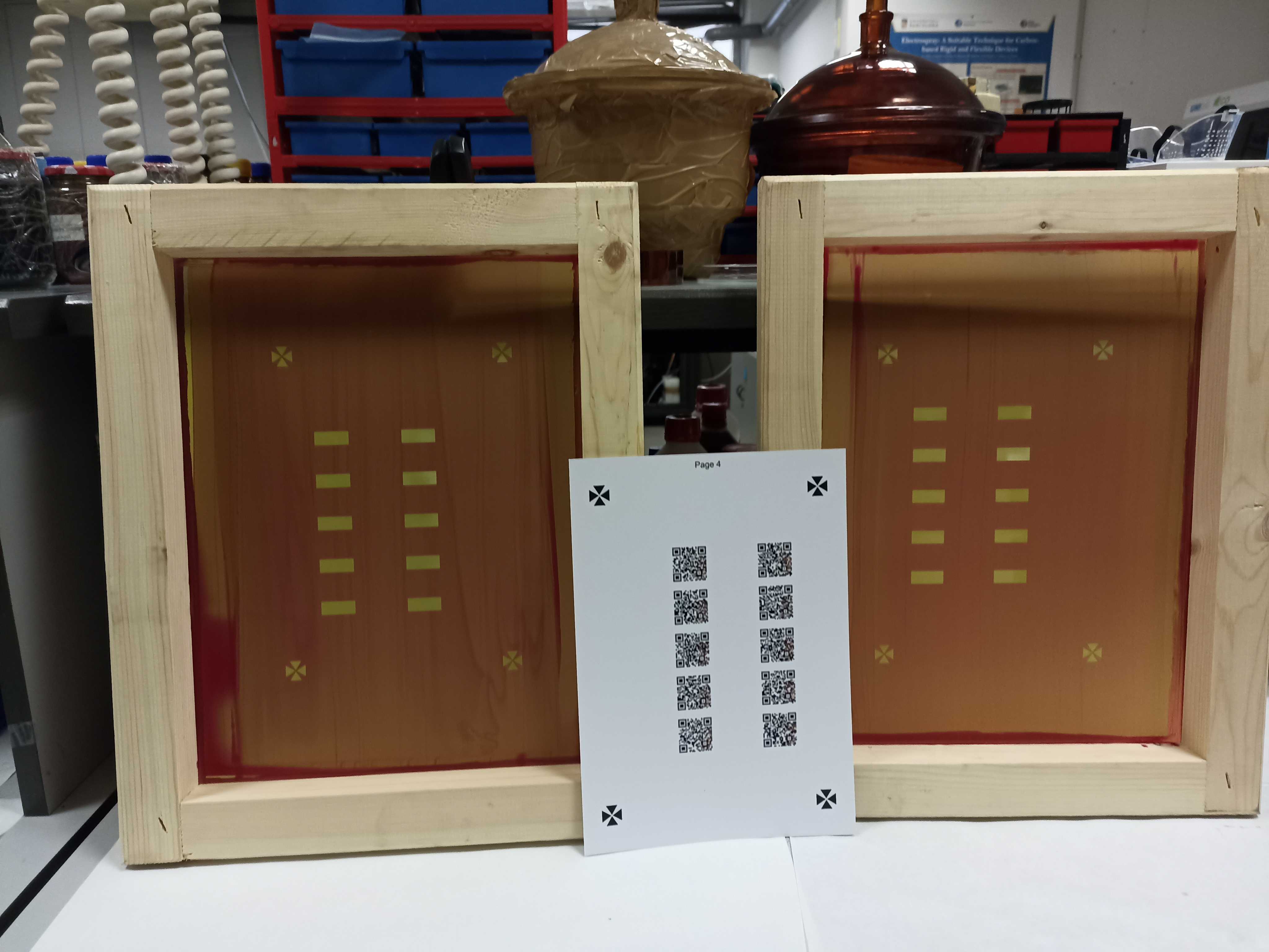
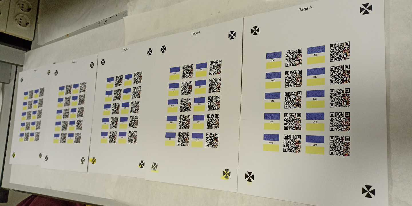
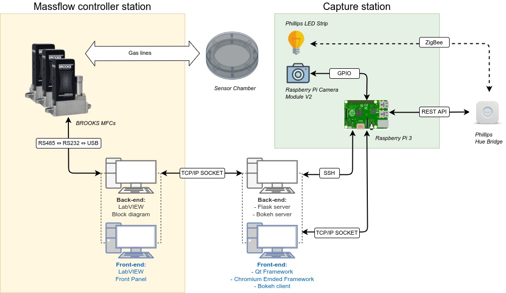
We designed and built our experimental setup from scratch. This experimental setup was used in the research of this thesis and related activities, e.g. seeking for new colorimetric indicators. The setup consisted of a complex system that responds to the necessity to capture colorimetric indicators targeting specific gases. Thus, the setup needed to solve not only the optical measurement, but also the management of target gas flows (see [fig:MGP_schema]).
The setup consisted of three main subsystems:
Mass-flow control station: a tiny desktop computer, a Lenovo ThinkCentre M93 Tiny, implemented the software to control up to five BROOKS 5850S mass-flow controllers [167], which fed a sensor chamber with the desired gas mix (see [fig:chamber_design]). The control over the BROOKS devices was done in LabVIEW [168].
Also, a LabVIEW front-end screen was implemented to enable user interaction in this subsystem. The tiny computer was equipped with a touchscreen to ease user interaction, but usually this station is set to automatic when using the setup to perform long-term data acquisition.
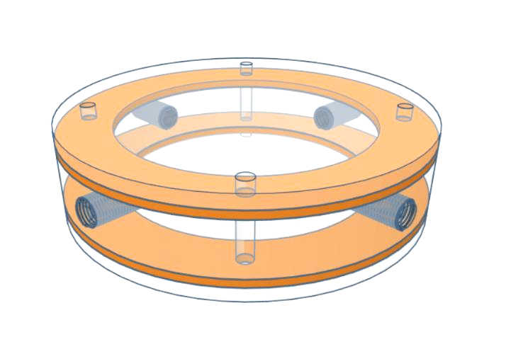
Moreover, LabVIEW used a serial communication protocol using the BROOKS official Windows DLL [169] with some hardware protocol adaptations (USB \(\Leftrightarrow\) RS232 \(\Leftrightarrow\) RS485).
Capture station: a single-board computer, a Raspberry Pi 3B+, implemented the software to control a digital camera (Raspberry Pi Camera v2) [135] and a strip of RGB LEDs from Phillips Hue [136] that acted as a variable light source.
Then, the control software of both the camera and the light strip was
implemented in Python [151]. Specifically, the
picamera module was used to drive the camera, and the
phue one to drive the LED strip 4.
User station: a desktop computer implemented the
user control software to manage all the system. This software was
implemented using Python again, but with a different stack in mind:
flask was used as a back-end service [170], and bokeh was
used to present plots in the front-end [171]. The front-end was based upon a
web-based technology that uses the popular Chromium Embedded Framework
to contain the main application [172].
The colorimetric indicator was exposed to a series of pulses of different controlled atmospheres. In total, it was exposed to \(\mathrm{15}\) pulses, \(\mathrm{100}\) minutes each, that consisted of exposing the sensor \(\mathrm{30}\) min to the target gas \(CO_2\), followed by an exposure of \(\mathrm{70}\) min to a clean atmosphere of synthetic air (\(\mathrm{21\%}\) oxygen, \(\mathrm{79\%}\) nitrogen). With this, the experiment lasted 25 hours.
Table 6.1 shows the expected concentration of the \(CO_2\) pulses versus the measured and corrected ones against dilution laws, as indicated by the manufacturer [167]. The target gas was diluted using synthetic air. We configured the experiment to repeat 3 times the same pulse for 5 different target concentrations: \(\mathrm{20\%}\), \(\mathrm{30\%}\), \(\mathrm{35\%}\), \(\mathrm{40\%}\) and \(\mathrm{50\%}\).
| Pulse | Expected [%] | Measured [%] |
|---|---|---|
| 1 | 20.0 | 25.21\(\ \pm \ \)0.00 |
| 2 | 20.0 | 25.22\(\ \pm \ \)0.22 |
| 3 | 20.0 | 25.22\(\ \pm \ \)0.22 |
| 4 | 30.0 | 36.62\(\ \pm \ \)0.22 |
| 5 | 30.0 | 36.67\(\ \pm \ \)0.31 |
| 6 | 30.0 | 36.67\(\ \pm \ \)0.31 |
| 7 | 35.0 | 42.10\(\ \pm \ \)0.40 |
| 8 | 35.0 | 42.30\(\ \pm \ \)0.40 |
| 9 | 35.0 | 42.20\(\ \pm \ \)0.40 |
| 10 | 40.0 | 46.90\(\ \pm \ \)0.40 |
| 11 | 40.0 | 47.30\(\ \pm \ \)0.40 |
| 12 | 40.0 | 47.40\(\ \pm \ \)0.40 |
| 13 | 50.0 | 57.60\(\ \pm \ \)0.50 |
| 14 | 50.0 | 57.60\(\ \pm \ \)0.50 |
| 15 | 50.0 | 57.60\(\ \pm \ \)0.50 |
These concentrations were selected as the \(CO_2\) indicator was designed to tackle the scenario of modified atmosphere packages (MAP) – \(\mathrm{20\%}\) to \(\mathrm{40\%}\) of \(CO_2\) – [32]. Also, this is why, the synthetic air was partially exposed to a humidifier to achieve proper work conditions for the colorimetric indicator, i.e. resembling a MAP containing some fresh food, like meet, fish or vegetable.
[fig:gas_pulses] shows a detailed view on the above-mentioned gas pulses, all the measures are shown for the target gas channel (\(CO_2\)), and both the dry and the humid synthetic air atmospheres (SA).
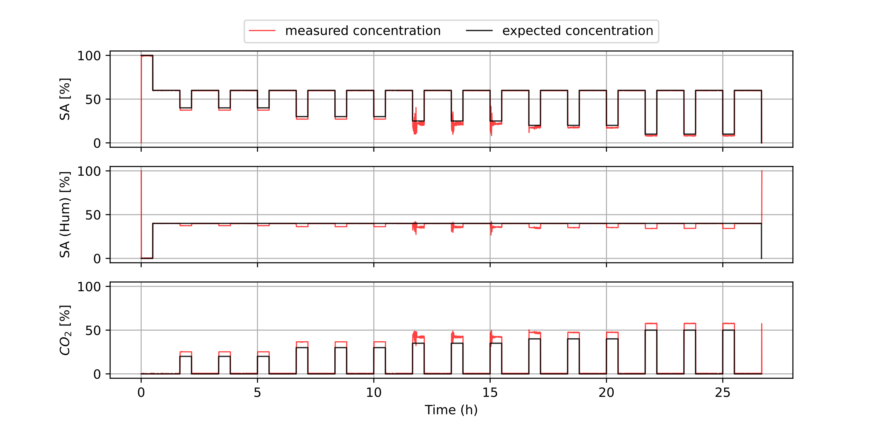
The sensor was exposed to different illumination conditions of white light. This was achieved using the above-mentioned Phillips Hue light system. Color temperatures ranged from 2500K to 6500K, in steps of 500K (see [fig:chamber_illuminants]). These are less aggressive light conditions than those we used in [ch:5] when studying the capacity of QR Codes in the colorimertry setup.
Also, the camera settings were fixed, without auto-exposition nor auto white-balance, to capture consistent images through all the dataset. This ensured we can extract the color reference tables during color correction only in the 9 first images.
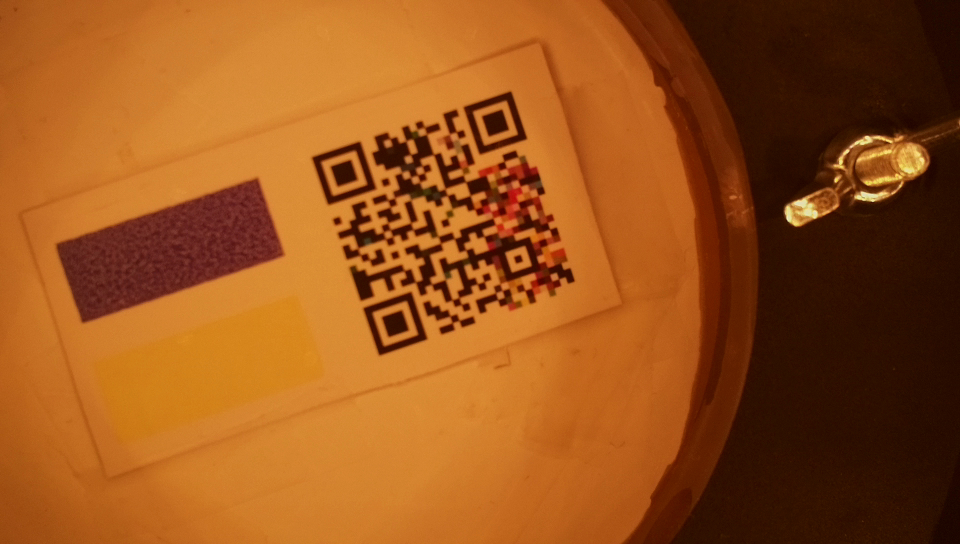
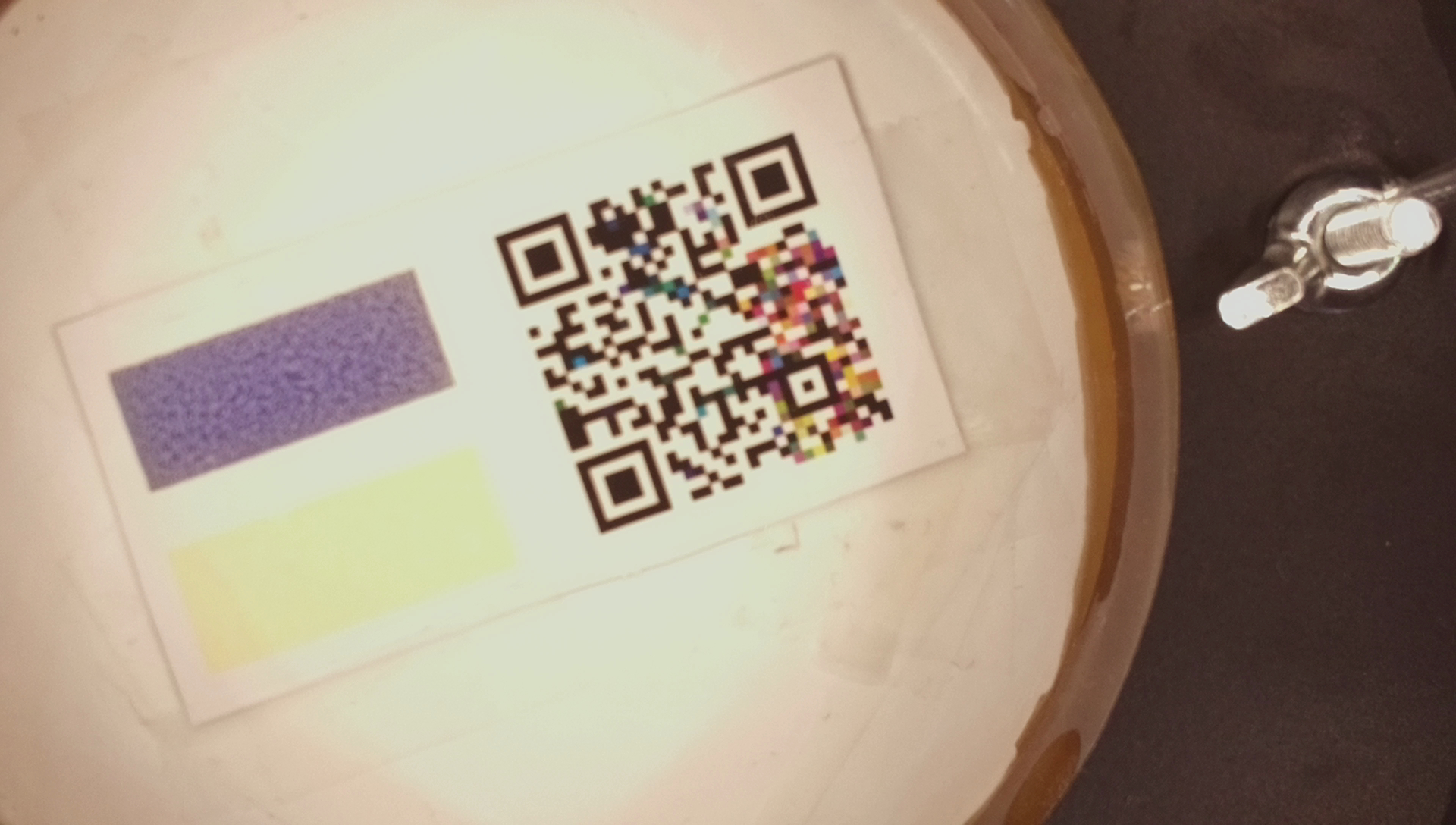
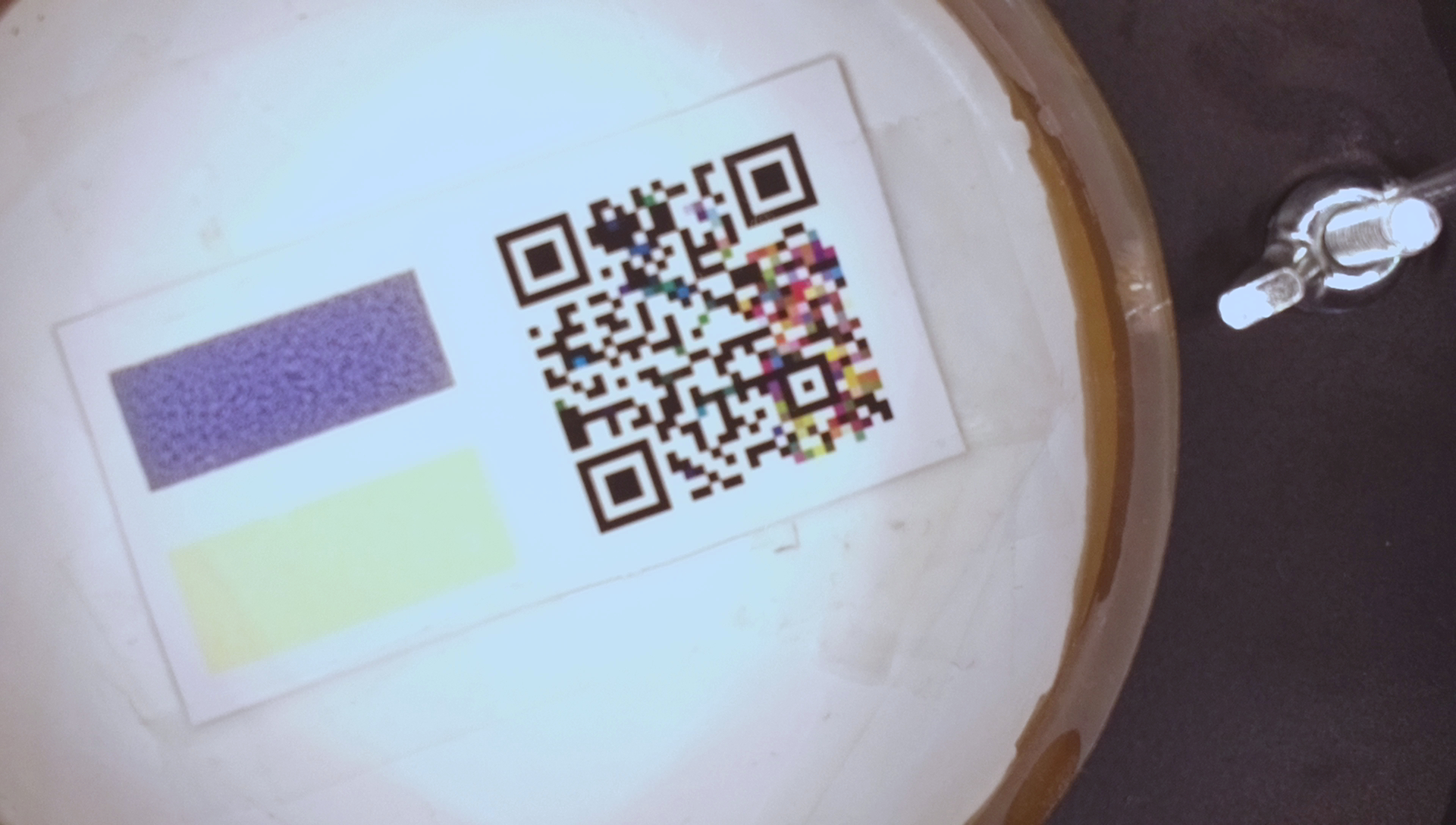
Notice, that the number of different light illuminations (9) was kept low to preserve an adequate sampling rate of the sensor response dynamics. Our setup performs the captures in a synchronous way: an image is taken, then the color illumination changes, then another image is taken, etc. The global sampling rate was \(\mathrm{1}\) FPS, which is the maximum frame rate a Raspberry Pi Camera can process at Full HD quality (\(\mathrm{1920 \times 1088}\) pixels). Then, the actual frame rate for each illumination stream was \(\mathrm{1/9}\) FPS.
In previous works, we already studied the relation between the colorimetric response of an indicator and the presence of the target gas [29], [30], [160], [163]. The relation we found was:
\[S [\%] = m \log(c) + n \label{eq:model}\]
where \(S\) is the colorimetric response of the sensor, \(c\) is the concentration of the target gas in the atmosphere, \(m\) and \(n\) are the constants of a linear law. Then, the colorimetric response is linear with the logarithm of the gas concentration. \(m\) represents the sensitivity towards the logarithm of the gas concentration, and \(n\) the response at very low concentrations.
Also, we can recover the sensitivity as a function of the gas concentration using derivates and use it to compute the error of the model for each concentration. To do so, we will use error propagation rules:
\[\left. \frac{\Delta S}{\Delta c} \right|_c = \frac{m}{c} \Longrightarrow \Delta c |_c = \Delta S |_c \cdot \frac{c}{m} \label{eq:sensitivity}\]
where \(c\) is a given concentration recovered with the inverted [eq:model], \(m\) depends on each fitted model, \(\Delta S |_c\) is the error of the measured signal response and \(\Delta c |_c\) is the model error for this given concentration.
Finally, the signal color response \(S [\%]\) is usually normalized following a metric. We defined this metric to resemble the normalization performed in an electronic gas sensor [30]. This kind of normalization divides the measured signal by the signal value assigned to the zero gas concentration, this produces a metric that is not upper-bounded \([0, \infty)\), the closer the initial resistance value is to zero, the greater the response. Let us adapt this normalization for a red channel of a colorimetric indicator:
\[S_r [\%] = 100 \cdot \frac{r(c) - r_0}{r_0 - r_{ref}} \label{eq:model_response}\]
where \(S_r\) is the response in % of the red channel, \(c\) the concentration of the target gas in %, \(r(c)\) the raw red sensor signal with an 8-bit resolution (0–255), \(r_0\) the value of \(r(c=0 \textrm{\%})\) and \(r_{ref}\) an absolute color reference which acts as the "zero resistance" compared to electronic sensors. For our sensor the value is \((r_{ref}, g_{ref}, b_{ref}) = (0, 0, 255)\), as our measured blue channel signal decreases when the gas concentration increases [31].
Let us start with the response of the colorimetric indicator under the different \(CO_2\) atmospheres. [fig:response_pulses] shows the signals obtained from the mean RGB channels for the colorimetric indicator for all the experiment captures in the D65 standard illuminant (6500K). In order to obtain these mean values, we created a computer vision algorithm to extract the region of interest. This algorithm was based on the state-of-the-art, presented in [ch:3], and our work, in [ch:4].
First, with these results, we could already confirm that we correctly selected our absolute reference to compute the color response, \((r_{ref}, g_{ref}, b_{ref}) = (0, 0, 255)\). As the previous works suggested [31], the color indicator moves from a blueish color to a yellowish color with the appearance of \(CO_2\) in the atmosphere.
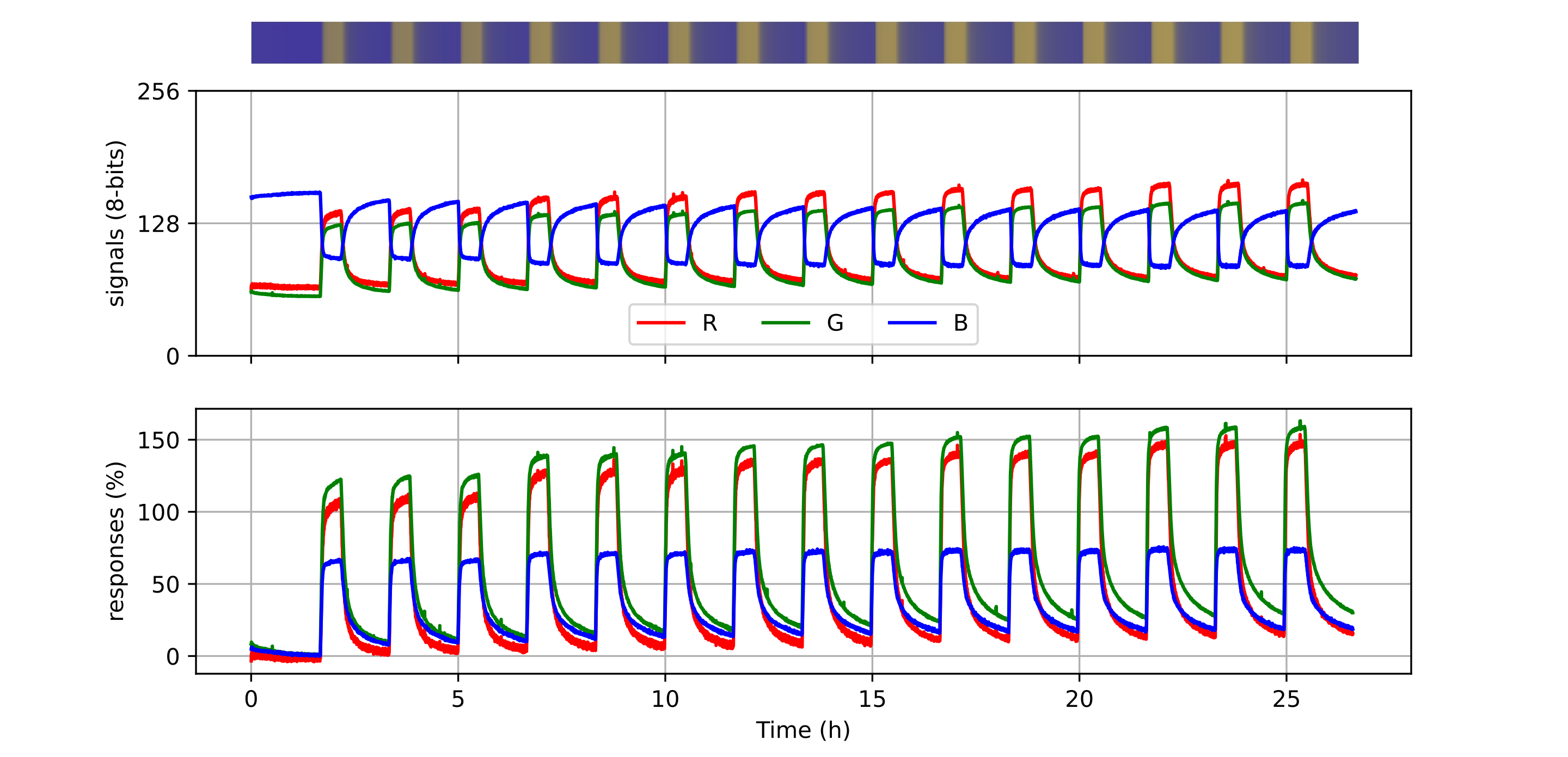
Then, [fig:response_pulses] displays the computed responses from the sensor. The responses were computed following [eq:model_response]. The results show the channel which achieved the best response was the green channel. This presented a higher response and less noise. Followed by the red channel, which performed close to the green channel in response, but with a more severe noise. The blue channel, performed with approximately the half of the response than the other channels at the lower concentration tested. And, its response saturated in the higher concentrations more rapidly than red and green channels.
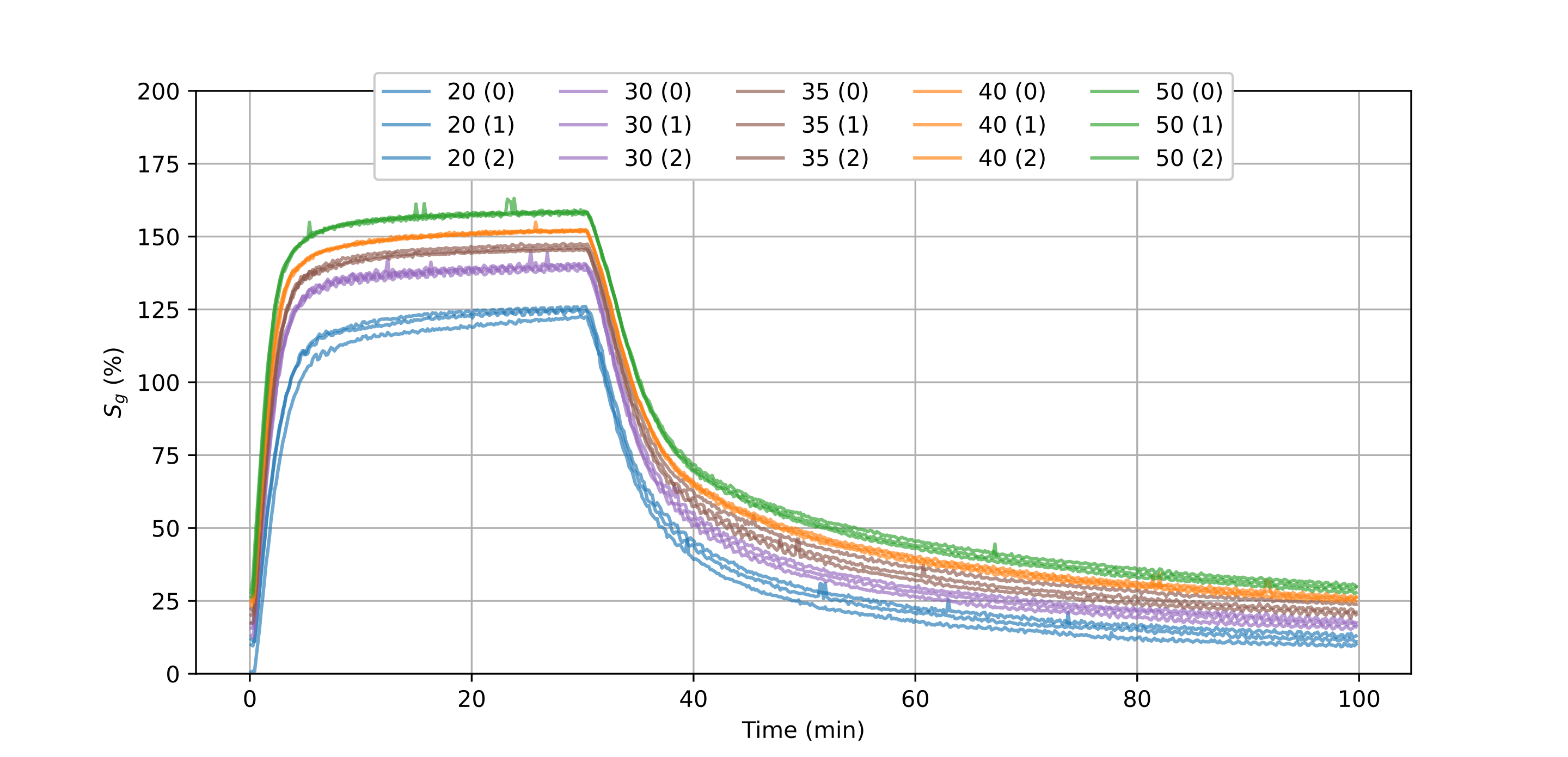
Moreover, in [fig:response_pulses_unified] we present the previous results but now stacked into the same time frame (the pulse duration of \(\mathrm{100}\) minutes). This is interesting from the gasometric standpoint. Our colorimetric indicator presented:
a fast response, achieving the \(\mathrm{90\%}\) of the \(S_g (\%)\) response in less than 5 minutes, for the highest concentration; and in less than 10 minutes, for the lowest one,
a reasonable maximum response above \(\mathrm{150\%}\) for the higher target concentration of \(CO_2\) \(\mathrm{50\%}\),
a slight saturation in the upper region of concentrations, this will be reflected in our fitted models,
good reproducibility among the replicas of each pulse, except for one pulse in the first triplet (\(\mathrm{20\%}\) of target gas concentration),
and, a drift in the lower concentration area, as pulses did not end in the same response they started.
All in all, [fig:response_pulses_unified] presented our colorimetric indicator as a good choice to detect the concentration of \(CO_2\) in modified atmosphere packaging (MAP). The caveats presented by the sensor: the saturation in the upper range (\(\mathrm{50\%}\)) and the drift in the lower range (\(\mathrm{0\%}\)) did not affect our further results as our models were targeting only to fit the data of the range that applies to MAP (\(\mathrm{20\%-50\%}\)).
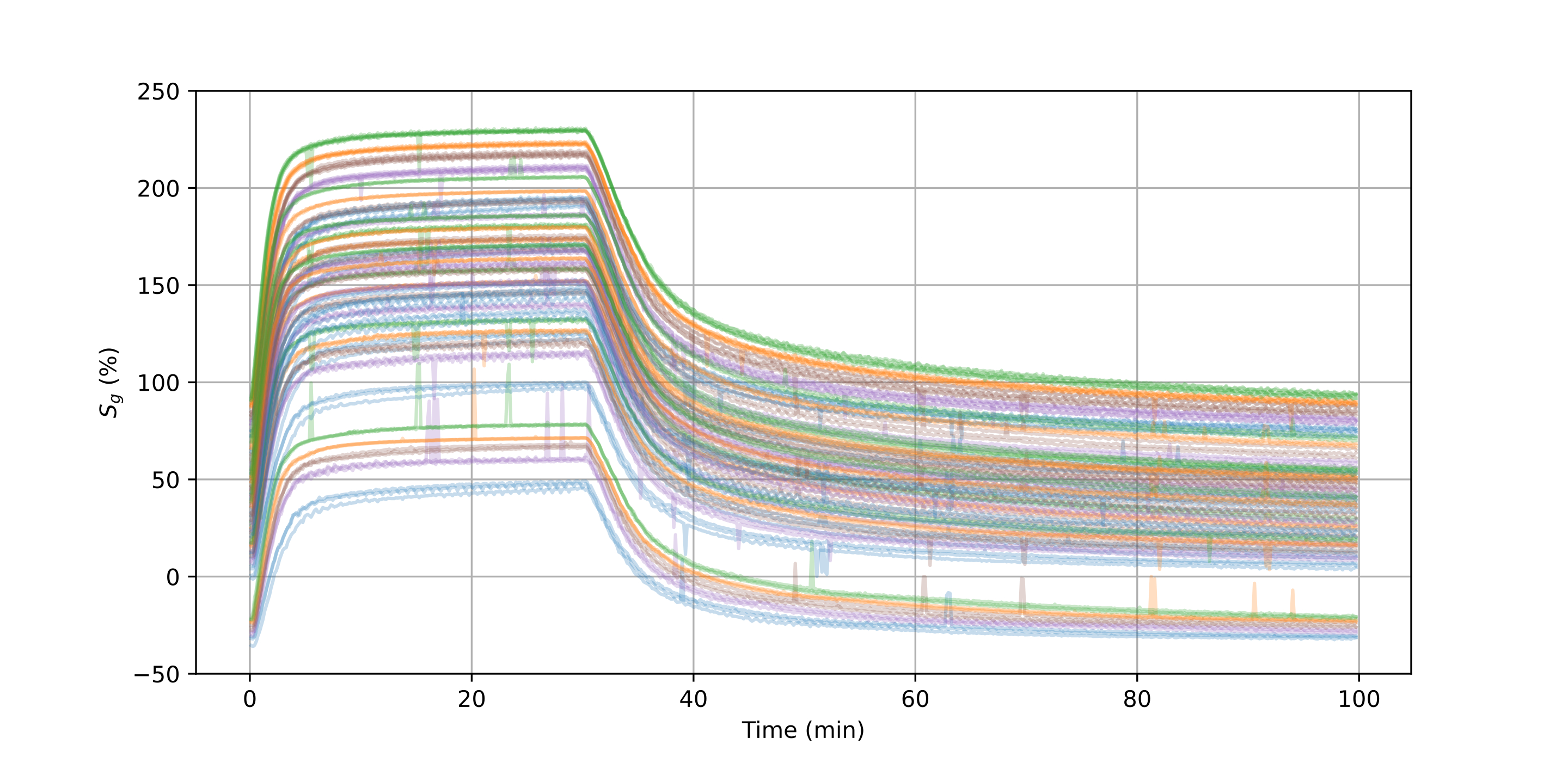
However, these results became meaningless when we exposed the colorimetric indicator to other light conditions than the D65 standard illumination, as the apparent sensor response changed drastically, as expected. [fig:response_pulses_unified_illuminations] portrays how the different illuminations affected the measure of the response for all the previous 15 pulses.
Finally, we exploited the color correction framework studied in [ch:6]. For each illumination, the 125 RGB colors placed inside the Color QR Code were extracted (see [fig:rgb_color_illuminations]). These colors were used to apply each one of the color correction techniques described in [ch:6] (see [tab:correctionssummary]). All the images from each illumination were corrected (>\(\mathrm{10000}\) image/illumination).
The references of the D65 standard illumination were taken as the reference color space of our correction techniques. [fig:response_pulses_unified_illuminations_corrected] shows how a TPS3 improved the situation presented in [fig:response_pulses_unified_illuminations] recovering a more suitable scenario to fit a colorimetric model to the data. In the next subsection, we focus in how we measured each pulse and fitting our proposed model to the different color corrections.
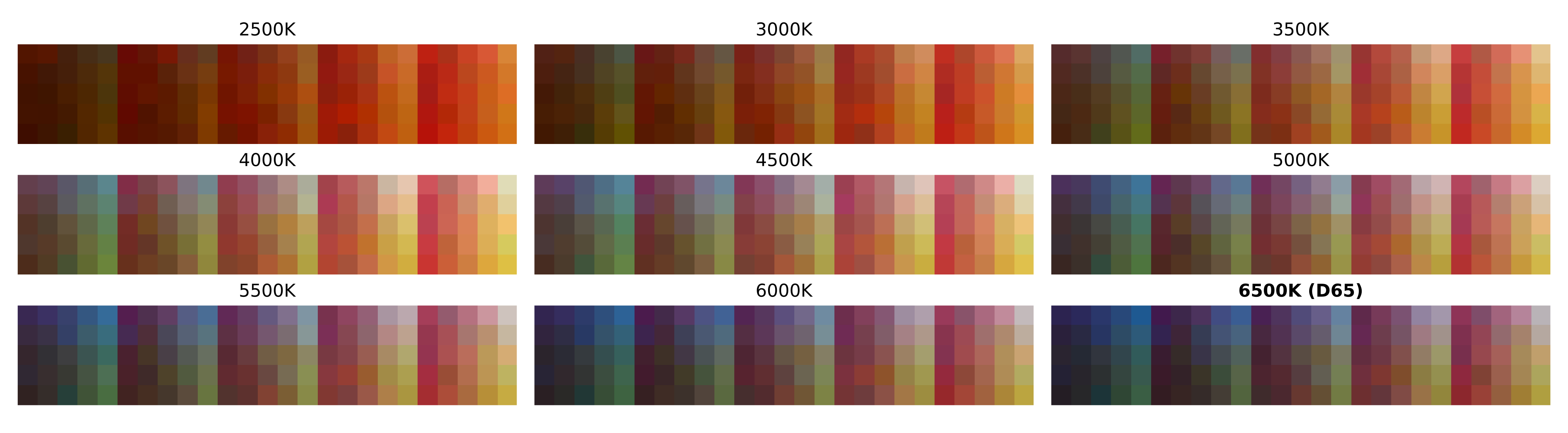
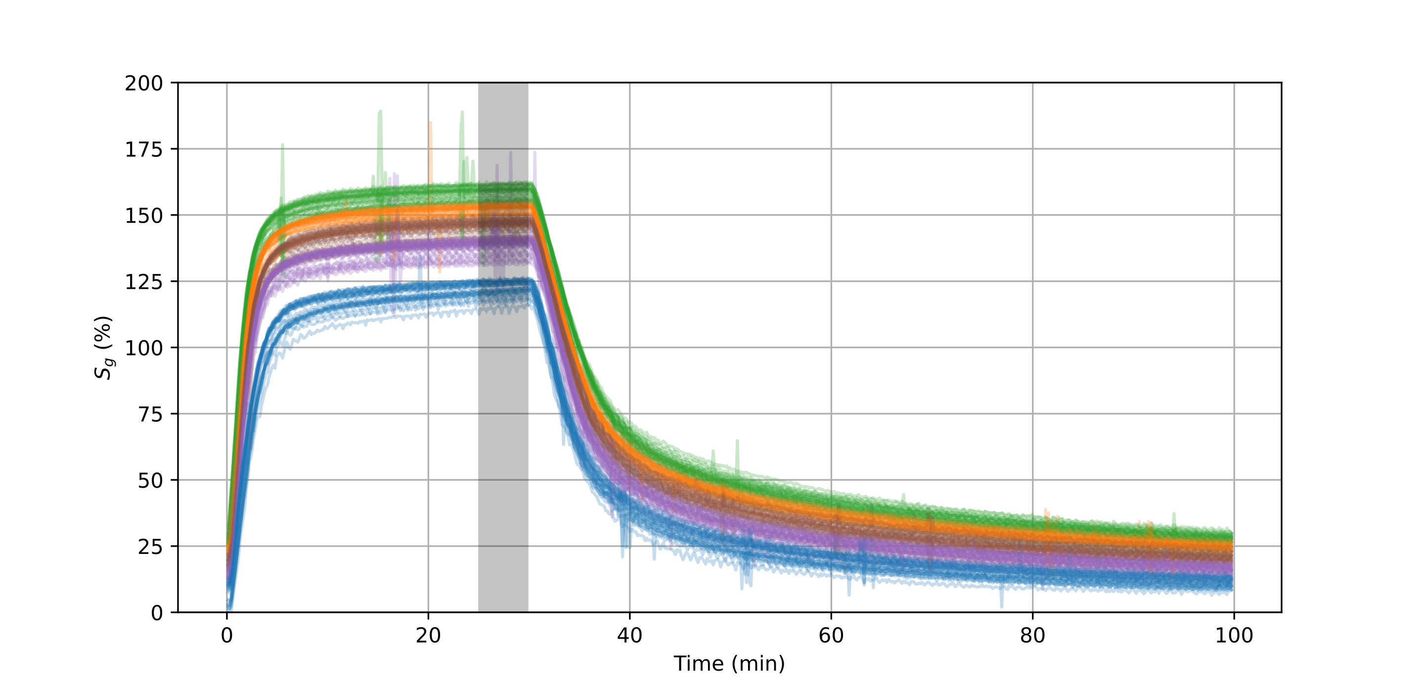
After applying the color correction techniques, we prepared the data to be suitable to fit our proposed linear-logarithmic model ([eq:model]). To do so we:
measured a mean corrected response value from the data during the last five minutes of gas exposition, ([fig:response_pulses_unified_illuminations_corrected] shows this time window shadowed),
transformed these response measures applying a logarithm,
linked those responses to their respective gas concentration measures from Table 6.1,
and, split the available data into train (75%) and validation subsets (25%).
Then we fed the train subsets, one for each available color correction in [tab:correctionssummary], to a linear model solver and obtained up to 22 different solutions, including the special NONE and PERF corrections described in [ch:6]. The validation subsets were used later to evaluate the models.
Let us start with these two reference corrections, [fig:model_NOPE_PERF] shows the fitting for both corrections, and [fig:model_NOPE_PERF_valid] shows the validation results. Results indicated that NONE was the worst case scenario, thus without correction the measurement of the colorimetric indicator was impossible. And PERF, as expected, was the best case scenario.
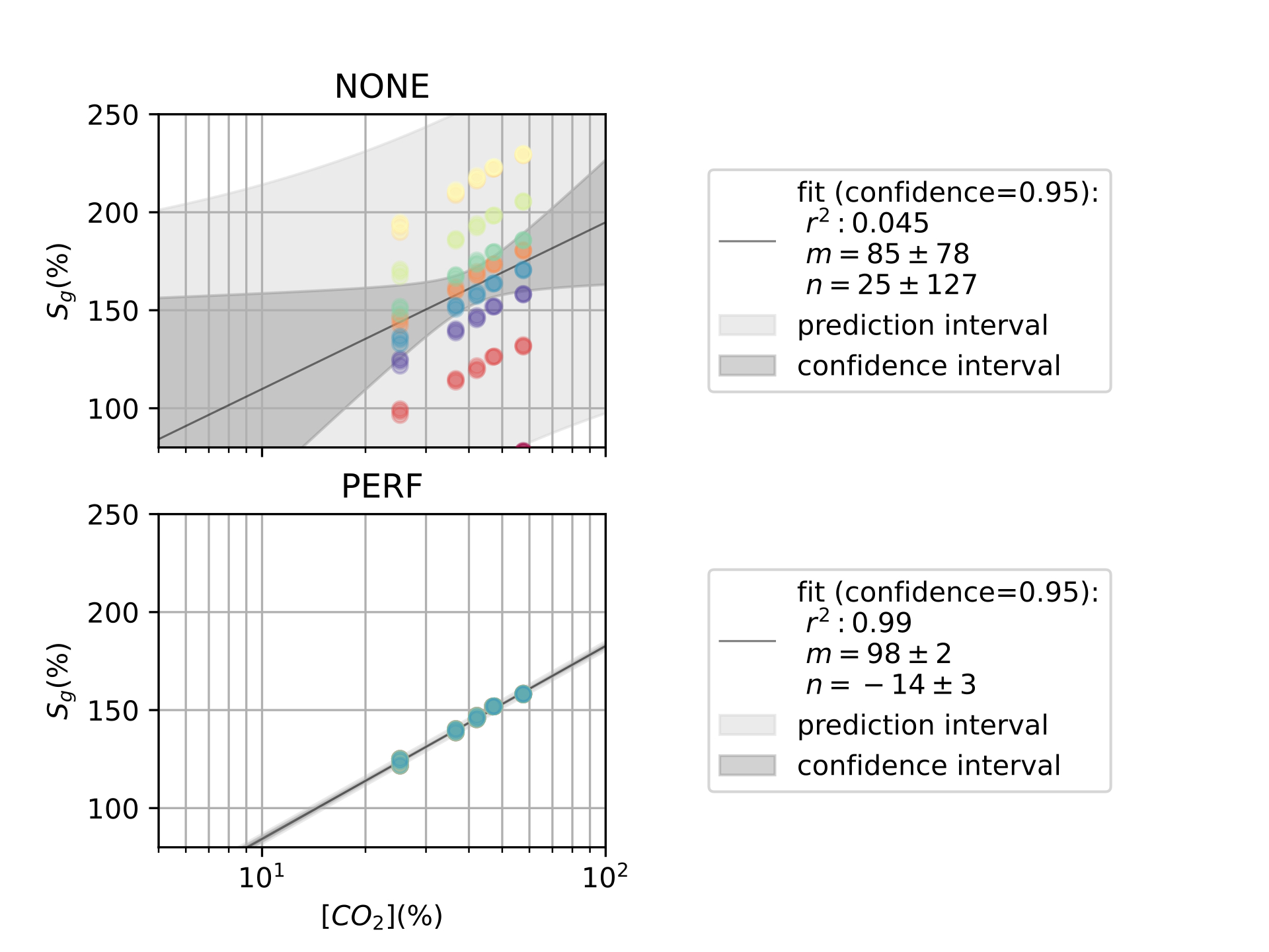
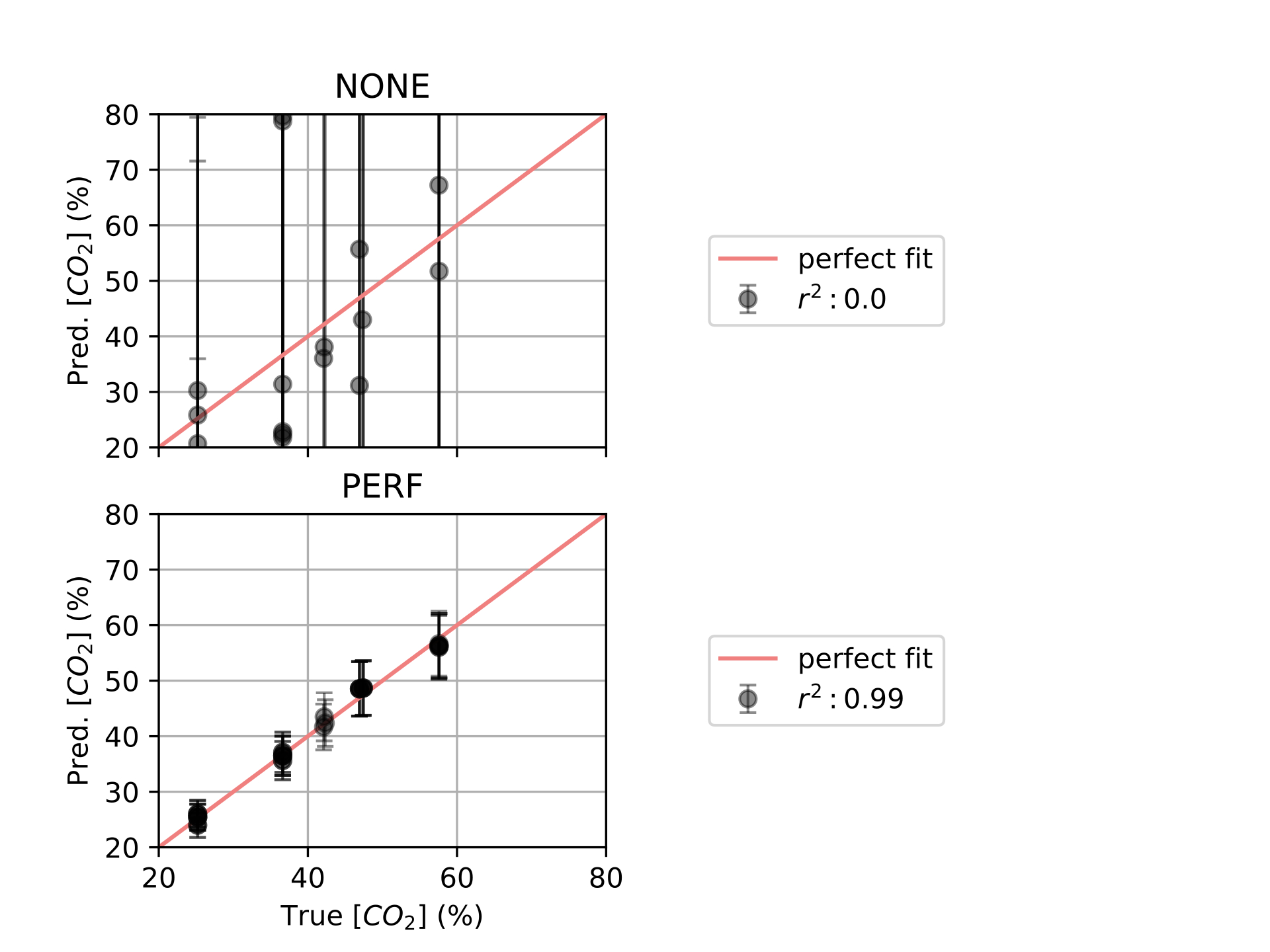
Specifically, when we say PERF is the best case scenario we mean the following: as the PERF model is the model of acquiring the data in a fixed setup –with a fixed camera configuration, a fixed light conditions, etc.–, the problem which we aim to solve in this thesis, the image consistency problem, is not present in this data. Therefore, it follows that the error seen in this model is the intrinsic error of the colorimetric indicator technology.
Then, the PERF results showed the good performance of the colorimetric indicator to sense \(CO_2\) in the target range of gas concentrations, scoring both \(r^2\) metrics for training ([fig:model_NOPE_PERF]) and validation ([fig:model_NOPE_PERF_valid]) almost a perfect score. This confirmed our model proposal.
Let us compare now the subsequent color corrections ([tab:correctionssummary]) with the before-mentioned extreme cases. The results are displayed from [fig:model_AFF] to [fig:model_TPS_valid]:
AFF: AFF0, AFF1 and AFF2 showed, in that order, the worst results in the dataset, both in training (see [fig:model_AFF]) and validation (see [fig:model_AFF_valid]). Although the experiment were biased towards this group of corrections. The bias is explained by the fact that we only changed color temperature of white illuminants in our setup.
However, AFF3 scored the best results above the whole other corrections groups, this is the correction which best approximated to the PERF solution.
This is explained again by the bias, but also because a general affine correction (AFF3) has contributions not present in a simple white-balance (AFF0, AFF1), like the cross-terms, or the affine without translation (AFF2). These contributions maximized the color correction quality by reducing the mean distance to corrected color of the sensor.
VAN: all corrections showed similar result to AFF3, but neither of them accomplished to outperform it. From the standpoint of the training model all four models showed the same fitting, if error correction is taken into account (see [fig:model_VAN]). From validation, the results showed also the same metric once again, good approaches to PERF (see [fig:model_VAN_valid]).
CHE: all corrections showed a similar result to AFF3 in training (see [fig:model_CHE]), the same as all VAN corrections. Only CHE0 showed a slightly worse metric in validation (see [fig:model_CHE_valid]), which is non-significant.
FIN: FIN0 presented similar results to AFF3 both in training (see [fig:model_FIN]) and validation (see [fig:model_FIN_valid]). However, FIN1, its root-polynomial version, presented worse results, both in training and validation. FIN2 and FIN3, the order 3 versions of FIN0 and FIN1, also failed to correct the color responses properly to fit the data.
TPS: all corrections showed good results, close to AFF3. In training, all the corrections showed the same fitting, if error correction is taken into account (see [fig:model_TPS]). As for validation, TPS0 and TPS1 achieved the best scores. (see [fig:model_TPS_valid]) Note here, TPS0 and TPS1 presented problems to ill-conditioned scenarios, this was solved using [eq:within_comparisom] criterion to detect and clean those scenarios.
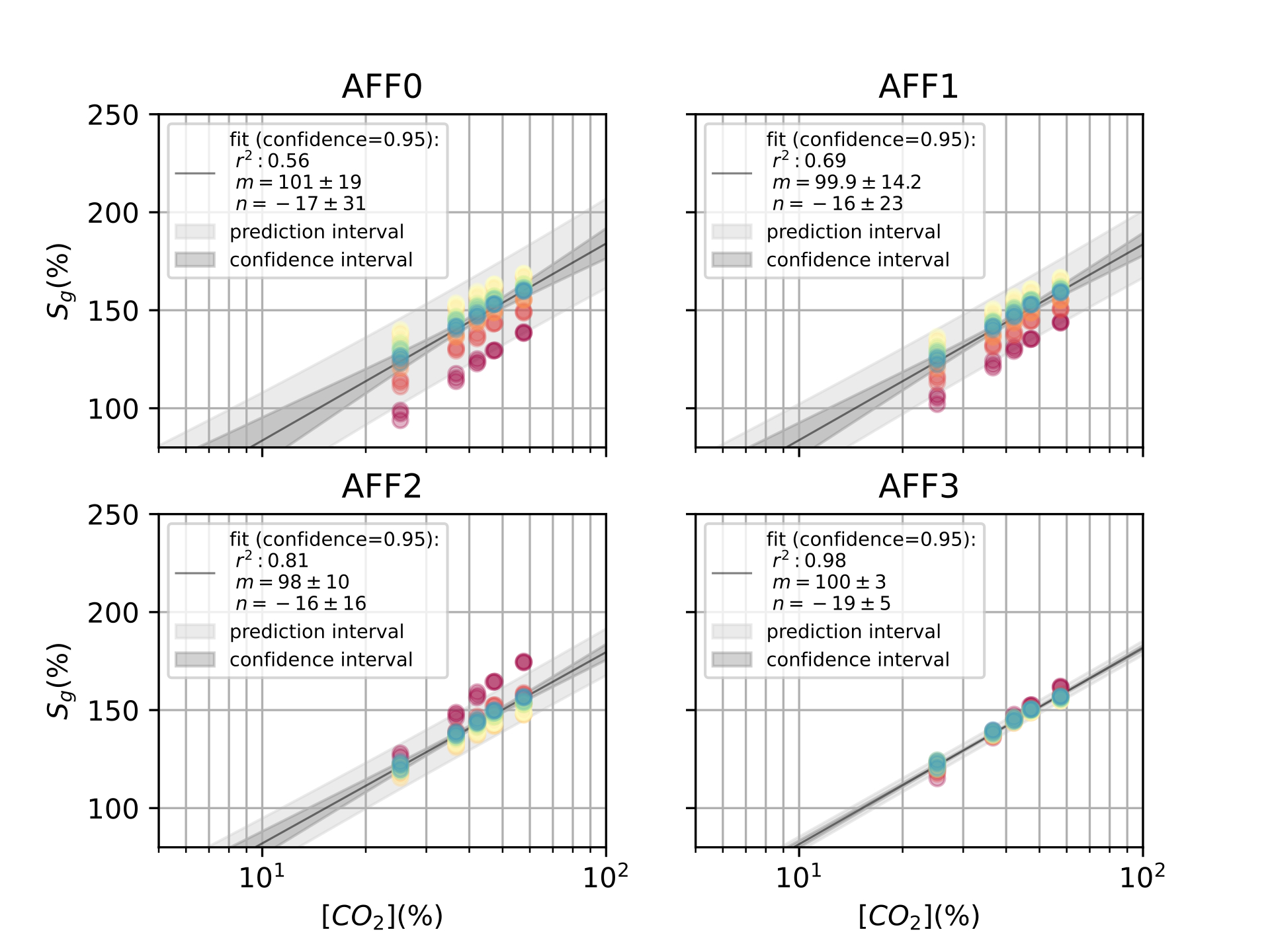
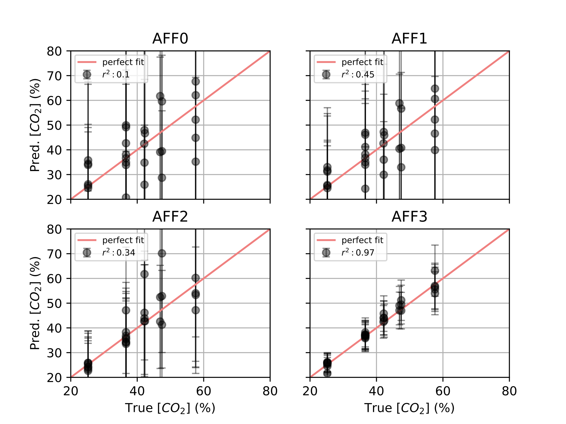
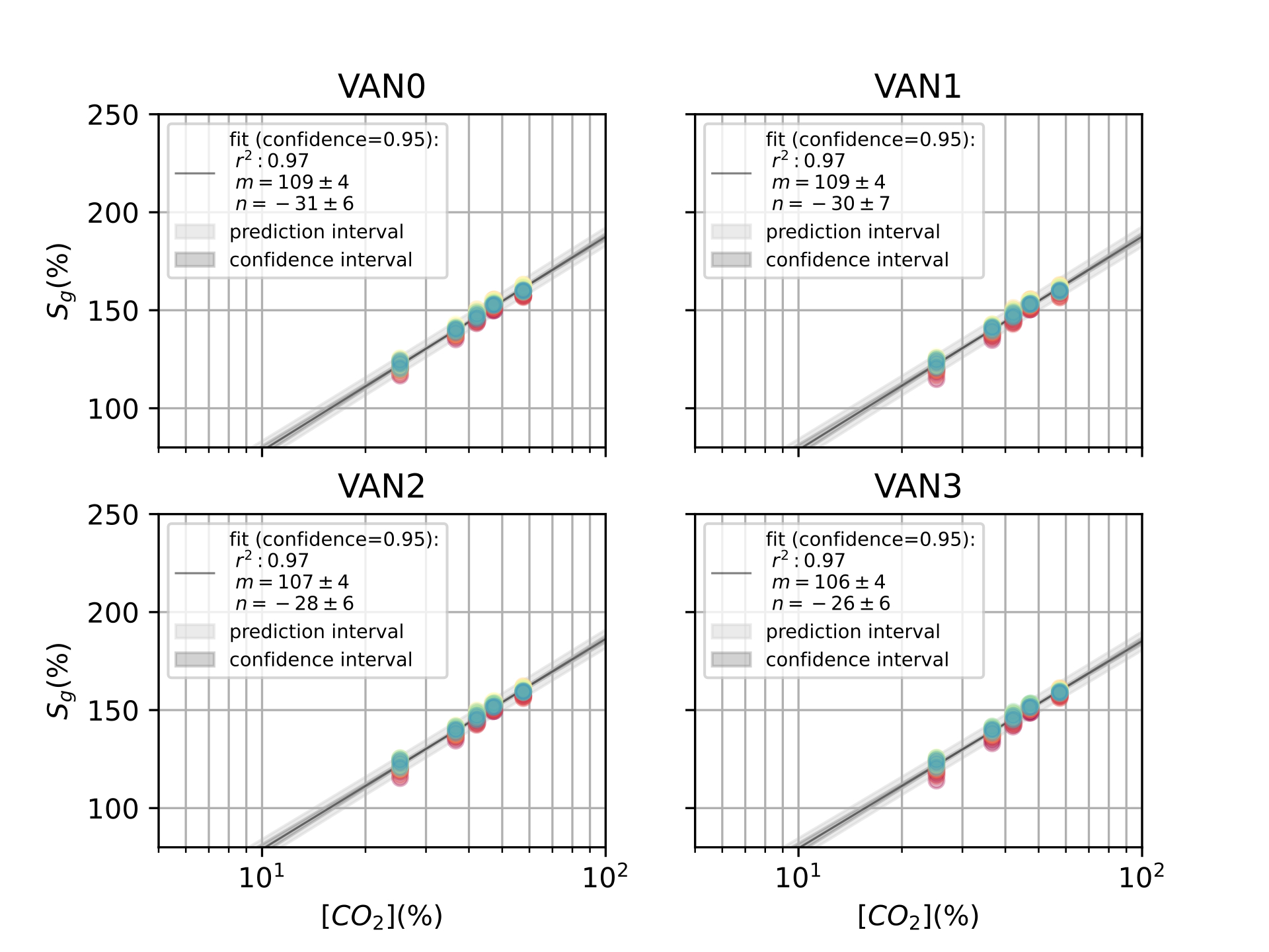
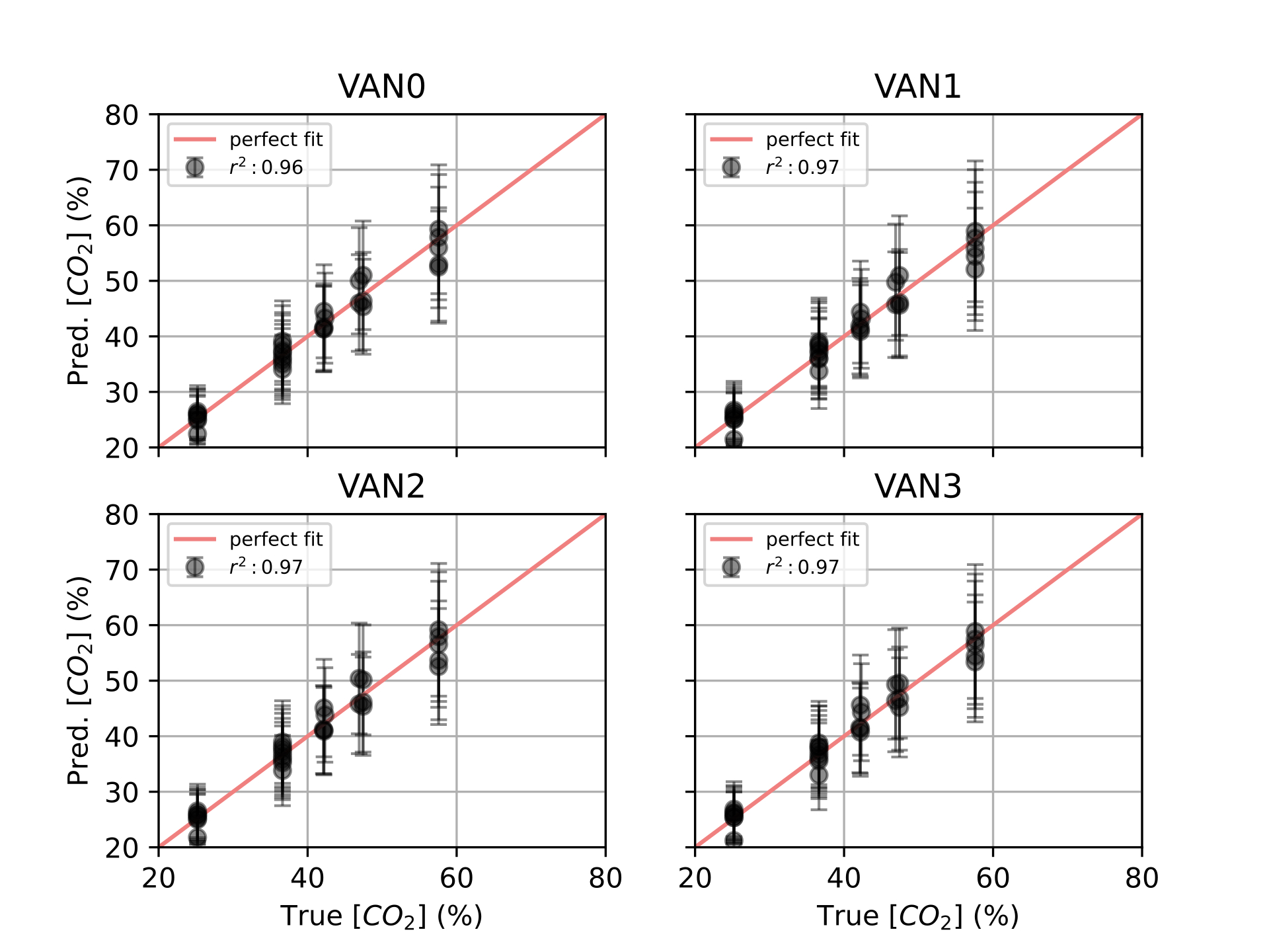
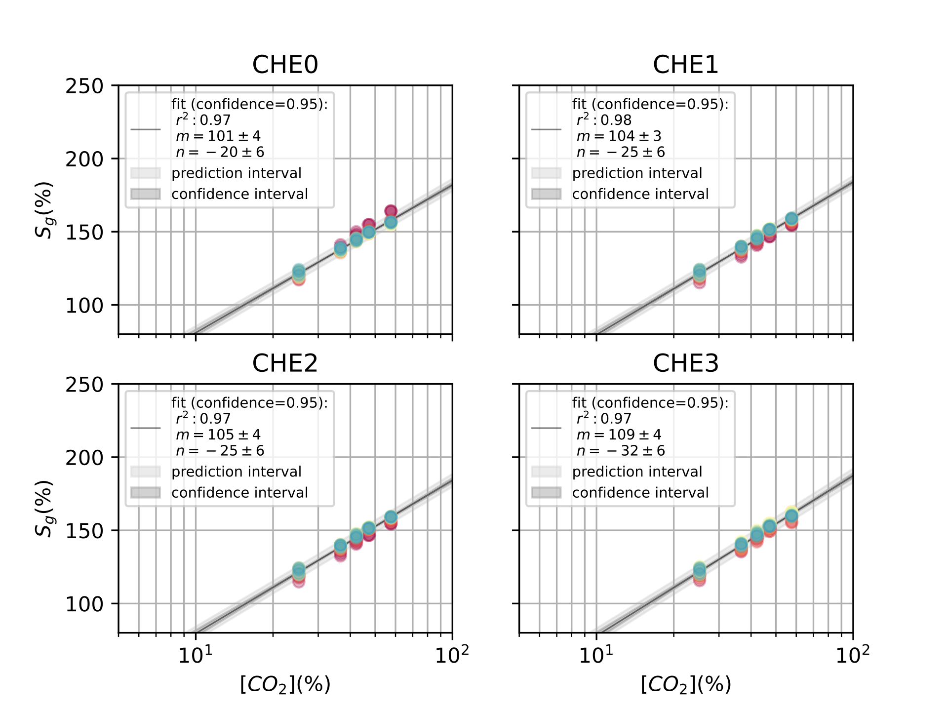
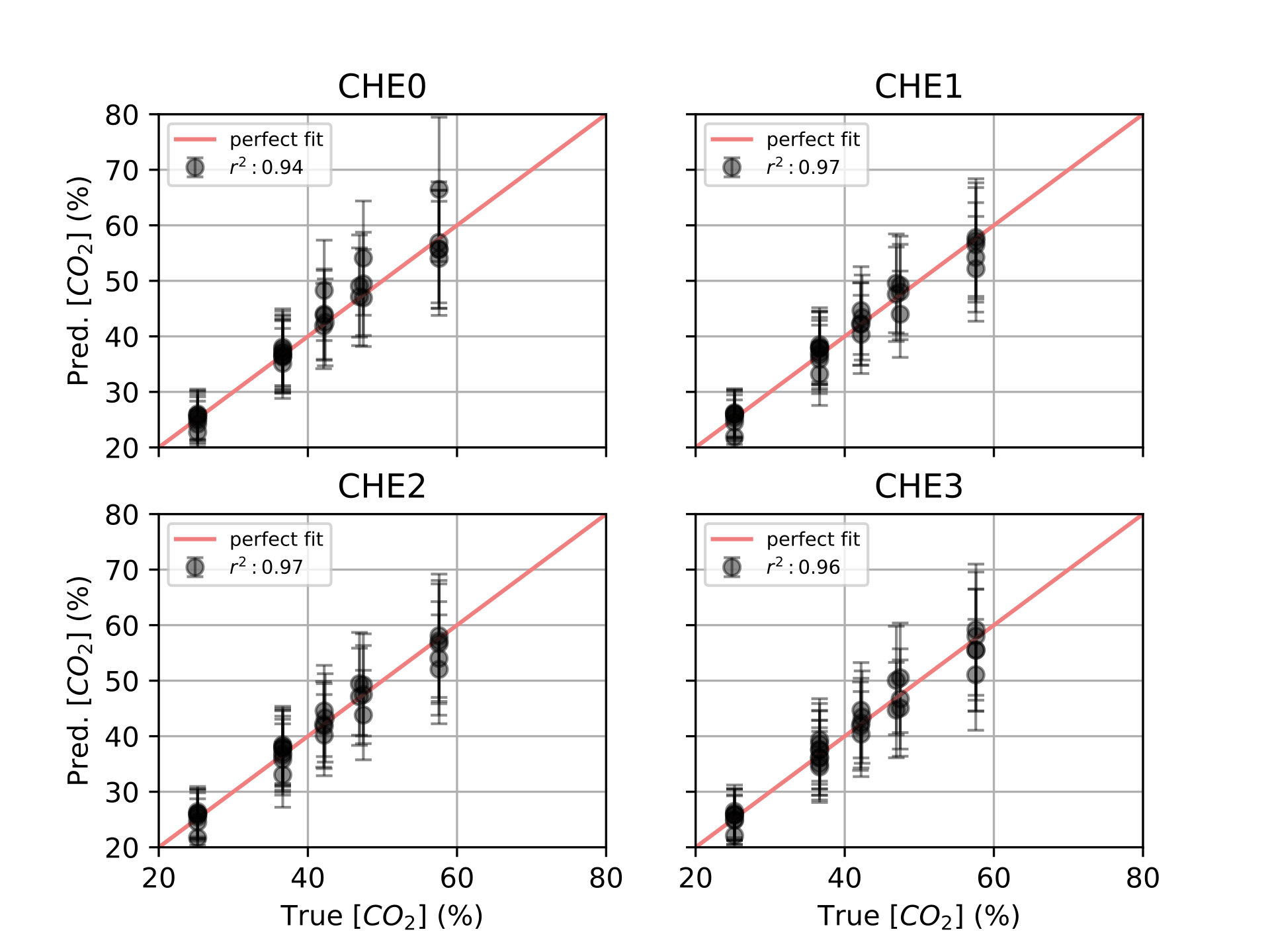
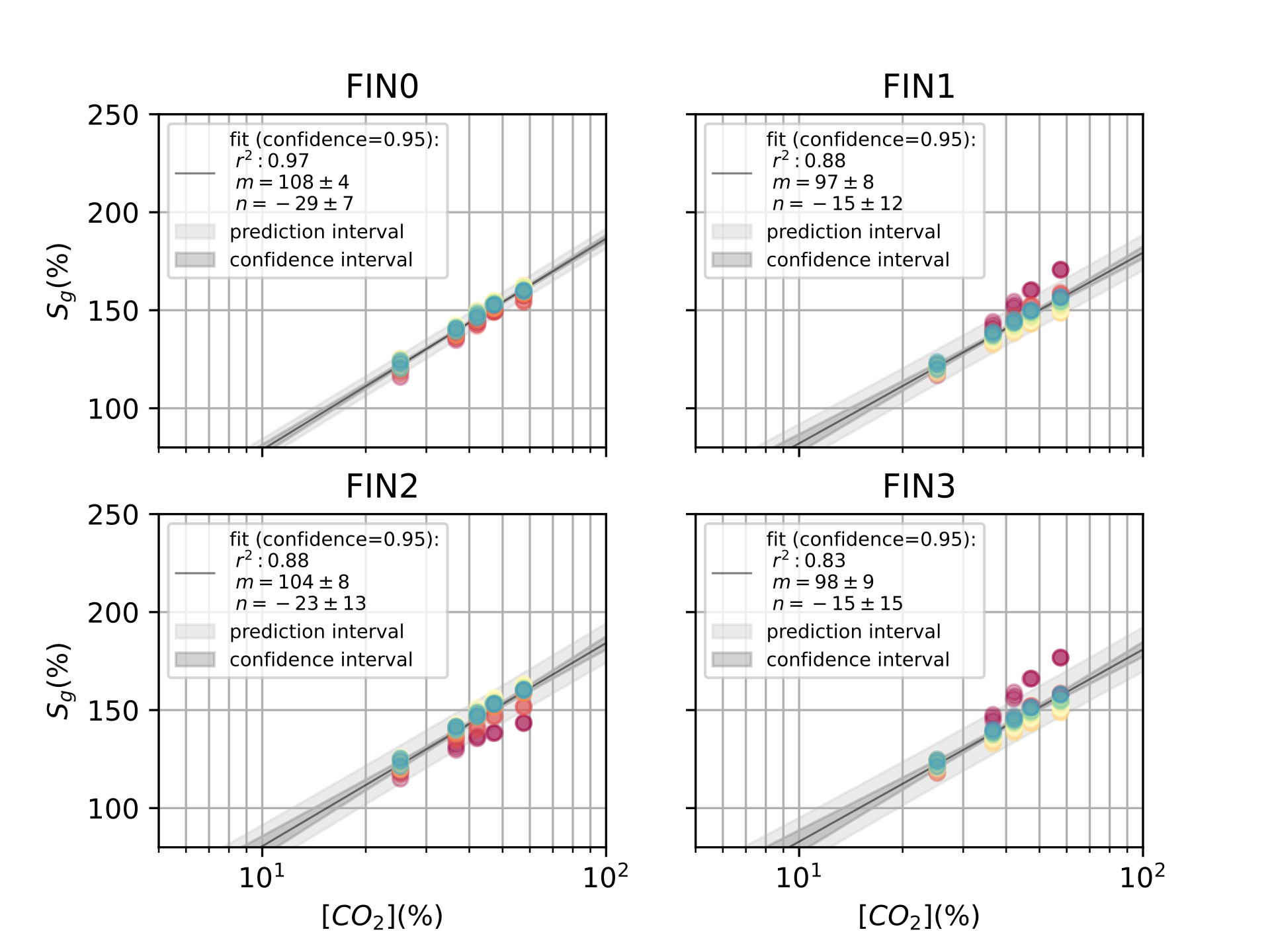
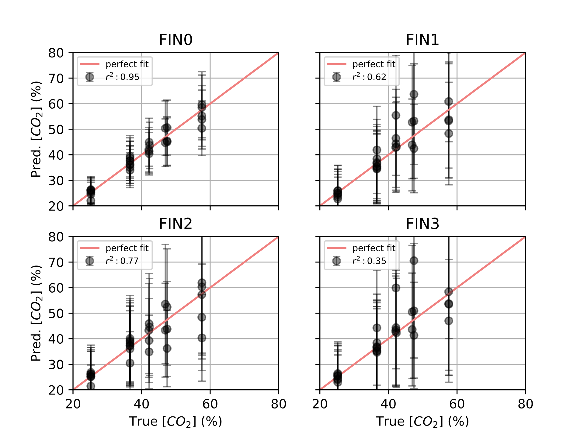
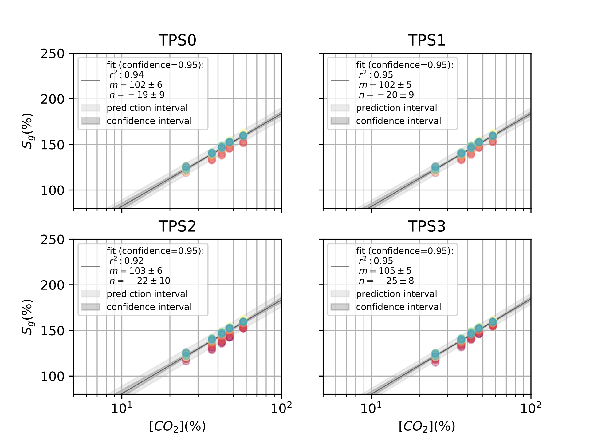
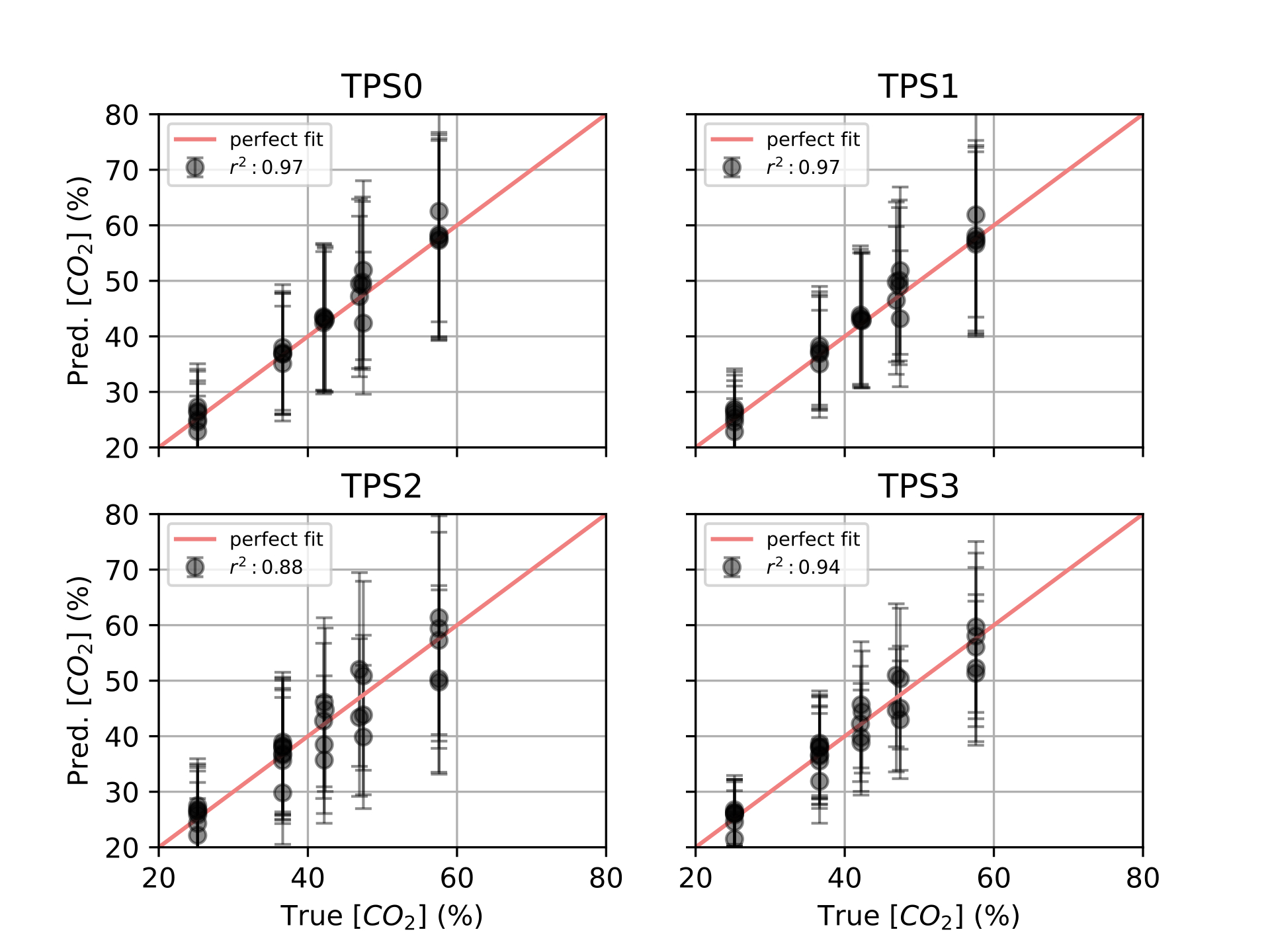
In this chapter, we demonstrated the application of our technology to colorimetric indicators. The process to design and acquire the signal of these colorimetric indicators was based upon our proposals of: Color QR Codes –[ch:4] and [ch:5]– and a color correction framework to solve the image consistency problem –[ch:6]–.
The studied example (\(CO_2\) colorimetric indicator [31]) presented an excellent response in the green channel of our measured data. Also, the red channel presented a good response, although it was noisy. The blue channel was discarded due to its reduced response.
Then, the studied colorimetric indicator presented good reproducibility and responded linearly with the logarithm of the concentration (for the PERF scenario), as we anticipated in other related work for other colorimetric indicators (such as \(NH_3\), \(H_2S\), etc.) [3], [29], [30], [159], [163].
Also, we tackled the problem of image consistency with our proposed framework. Results indicated that the NONE correction model (without applying any color correction) was useless. We correctly applied the AFF, VAN, CHE, FIN and TPS corrections. We even detected corner cases of ill-conditioned color corrections in TPS0 and TPS1 using the criteria defined in the previous chapter.
Furthermore, AFF3 outperformed all corrections, which approximated the PERF scenario with the best \(r^2\) scores both in training and validation. This was somehow expected as the problem was biased towards a white-balancing problem, as we used only white light sources from 2500K to 6500K color temperature in our experiments. Despite this, we demonstrated that AFF0 or AFF1, the most common white-balance corrections, were not enough to color correct the data. On one hand, VAN, CHE and TPS followed the results of AFF3 quite close, remaining in reserve for further analysis in more extreme illumination conditions. On the other hand, FIN presented the worse results (other than AFF0, AFF1 and AFF2), this correlates with [ch:6] conclusions, where we found that the lack of translation components in the color correction, produced poor results for FIN corrections.
All in all, [tab:resultssummary7] summarizes the model results displayed from [fig:model_NOPE_PERF] to [fig:model_TPS_valid]. In the table, we also added four additional metrics: the \(\Delta c\) (see [eq:sensitivity]) at 20% and 50% gas concentration and their respective relative metrics, namely the relative error \(\upepsilon_c\) of our model in those gas concentrations.
This summary highlights the above-presented evidence. The \(CO_2\) color indicator presented around 10% of relative error in the studied range (\([CO_2] = 20\% - 50\%\) ) by itself (PERF). As reference, a commercial electronic \(CO_2\) sensor from Sensirion has a \(\mathrm{3\%}\) relative error [173].
Also, without color correction (NONE), it presented a \(\mathrm{440\%}\) relative error, which is a useless result. Moreover, only correcting with white-balance (AFF0, AFF1) scored around \(\mathrm{70-90\%}\) relative error. Only AFF3 and related corrections (VAN, CHE) scored good results within \(\mathrm{10-20\%}\). TPS methods scored slightly worse results in the range of \(\mathrm{20-30\%}\) relative error. Then, our result is an excellent result for cost-effective disposable sensors, which are not meant to be persistent
Finally, seeking for improving these results, let us discuss some future work for this chapter.
First, in this chapter, we concluded that AFF3 was the best correction to color correct the presented color indicator for \(CO_2\) sensing. As mentioned, this was probably a biased dataset towards this kind of color deformation. We should look for more complex illumination configurations to enhance the dataset here presented. We already used those kinds of extreme light configuration in [ch:5] when we created the Color QR Codes.
Second, we could also modify the camera capturing settings, this is an interesting topic, as the image consistency problem is not only affected by the light source but also by the camera. Going further, we could perform captures with several devices at the same time. All these new approaches to the problem require more complex setups.
Third, in [ch:6] we concluded we ought to use more locally-bounded color references to specific problems, such the problem of colorimetric indicators. However, when we introduced this chapter we explained that we broaden the amount of encoded colors (from [29] to [30]) instead of keeping them to a representative subset of the RGB color spaces that was representative of the problem. Both statements are compatible.
As explained before, we failed to obtain the proper representative colors of the problem due to a color reproduction problem, thus we broadened the color chart to a general-purpose 125 RGB colors, to obtain an equidistributed sample of the printer colors. In order to close the loop, as suggested in [ch:6], now that we have more than 24 colors ([ch:6], ColorChecker) we should implement newer color corrections, based only on those color references that are representative of our data –i.e. the nearest colors–, and seek for an improvement of the results, specially in the TPS color corrections.
| Correction | \(\mathbf{m \left[\frac{\%}{\%}\right]}\) | \(\mathbf{n [\%]}\) | \(\mathbf{r^2 [-]}\) | \(\mathbf{r_{valid}^2 [-]}\) | \(\mathbf{\Delta c_{20} [\%]}\) | \(\mathbf{\Delta c_{50} [\%]}\) | \(\mathbf{\upepsilon_{20} [\%]}\) | \(\mathbf{\upepsilon_{50} [\%]}\) |
|---|---|---|---|---|---|---|---|---|
| NONE | 90\(\ \pm \ \)80 | 200\(\ \pm \ \)130 | 0.04 | 0.00 | 88 | 249 | 440 | 497 |
| PERF | 98\(\ \pm \ \)2 | -14\(\ \pm \ \)3.0 | 0.99 | 0.99 | 2 | 5 | 9 | 10 |
| AFF0 | 101\(\ \pm \ \)19 | -17\(\ \pm \ \)31 | 0.56 | 0.10 | 18 | 51 | 90 | 102 |
| AFF1 | 100\(\ \pm \ \)14 | -16\(\ \pm \ \)23 | 0.69 | 0.45 | 14 | 38 | 68 | 77 |
| AFF2 | 98\(\ \pm \ \)10 | -16\(\ \pm \ \)16 | 0.81 | 0.34 | 10 | 27 | 48 | 55 |
| AFF3 | 100\(\ \pm \ \)3 | -19\(\ \pm \ \)5 | 0.98 | 0.97 | 3 | 8 | 14 | 16 |
| VAN0 | 109\(\ \pm \ \)4 | -31\(\ \pm \ \)6 | 0.97 | 0.96 | 3 | 10 | 17 | 19 |
| VAN1 | 109\(\ \pm \ \)4 | -30\(\ \pm \ \)7 | 0.97 | 0.97 | 4 | 11 | 19 | 21 |
| VAN2 | 107\(\ \pm \ \)4 | -28\(\ \pm \ \)6 | 0.97 | 0.97 | 3 | 10 | 17 | 20 |
| VAN3 | 106\(\ \pm \ \)4 | -26\(\ \pm \ \)6 | 0.97 | 0.97 | 4 | 10 | 18 | 20 |
| CHE0 | 101\(\ \pm \ \)4 | -20\(\ \pm \ \)6 | 0.97 | 0.94 | 3 | 9 | 17 | 19 |
| CHE1 | 103\(\ \pm \ \)4 | -25\(\ \pm \ \)6 | 0.98 | 0.97 | 3 | 9 | 16 | 18 |
| CHE2 | 105\(\ \pm \ \)4 | -25\(\ \pm \ \)6 | 0.97 | 0.97 | 3 | 9 | 17 | 19 |
| CHE3 | 109\(\ \pm \ \)4 | -32\(\ \pm \ \)6 | 0.97 | 0.96 | 3 | 10 | 17 | 20 |
| FIN0 | 108\(\ \pm \ \)4 | -29\(\ \pm \ \)7 | 0.97 | 0.95 | 4 | 11 | 19 | 21 |
| FIN1 | 97\(\ \pm \ \)8 | -15\(\ \pm \ \)12 | 0.88 | 0.62 | 7 | 21 | 37 | 42 |
| FIN2 | 104\(\ \pm \ \)8 | -23\(\ \pm \ \)13 | 0.88 | 0.77 | 8 | 22 | 38 | 43 |
| FIN3 | 98\(\ \pm \ \)9 | -15\(\ \pm \ \)15 | 0.83 | 0.35 | 9 | 26 | 46 | 52 |
| TPS0 | 102\(\ \pm \ \)6 | -19\(\ \pm \ \)9 | 0.94 | 0.97 | 5 | 15 | 27 | 31 |
| TPS1 | 102\(\ \pm \ \)5 | -20\(\ \pm \ \)9 | 0.95 | 0.97 | 5 | 14 | 26 | 29 |
| TPS2 | 103\(\ \pm \ \)6 | -22\(\ \pm \ \)10 | 0.92 | 0.88 | 6 | 17 | 30 | 33 |
| TPS3 | 105\(\ \pm \ \)5 | -25\(\ \pm \ \)8 | 0.95 | 0.94 | 4 | 13 | 22 | 25 |
This thesis tackled the problem of acquiring data in a quantitative manner from colorimetric indicators, and other colorimetric applications. To do so, the problem of automating color calibration ought to be resolved with a seamless integration with the colorimetric application, without any additional barriers to the final consumer, thus using well-known 2D barcodes.
Here, we present a summary of the main conclusions for each one of the thesis objectives:
To capture machine-readable patterns placed on top of challenging surfaces. Results demonstrated that our method performed better than other extraction methods. We proved so by using the same commercial QR Code reader (ZBar) on the same image, which had been corrected by the proposed methods (AFF, PRO, CYL and TPS) for our three datasets (SYNT, FLAT and SURF), and computing a data readability factor \(\mathcal{R}\) for each method and dataset.
For the SYNT and FLAT datasets our method scored similar to the previous methods with almost a \(\mathcal{R}=100\%\), for the SURF dataset –where challenging surfaces were prsent–, AFF and PRO methods scored really poor results, a \(\mathrm{0\%}\) and \(\mathrm{2\%}\), respectively. CYL method scored a \(\mathrm{50\%}\), and TPS up to \(\mathrm{79\%}\).
By combining both CYL and TPS methods, we arrived to a joint result of \(\mathrm{84\%}\). We even benchmarked this against ZBar without any image correction. This proved that our method (TPS+CYL) scored 4 times better than a bare ZBar decoding (\(\mathrm{84\%}\) vs \(\mathrm{19\%}\)).
To define a back-compatible QR Code modification to extend QR Codes to act as color charts. Results indicated that our method minimized the error applied to a QR Code when color is present, both SNR and BER figures demonstrated that for any of the channels considered. We also demonstrated that the data zone (D) is the most suitable one to embed color references, as it presents a higher resilience to be manipulated.
Our method outperformed a random placement of colors by far. For example, for a version 5 QR Code, our method outperformed by a \(\mathrm{150\%}\) the results of the random assignment method for the data zone; and almost a \(\mathrm{500\%}\) for the global EC&D zone, embedding more than \(\mathrm{300}\) colors in one QR Code.
To achieve image consistency using color charts for any camera or light setup, enabling colorimetric applications to yield quantitative results. Results proved that all TPS methods are the best methods both in \(\overline{\Delta_{RGB}}_{within}\) and \(\overline{\Delta_{RGB}}_{inter}\) metrics, scoring half or less the distance of the nearest competitor, the general AFF correction.
Despite this, the original TPS3D method presented a huge number of ill-conditioned cases where the image was not properly corrected, around the \(\mathrm{20\% - 30\%}\) of the cases. This ill-conditioned scenarios were solved when imposing our smoothness proposal.
Also, results indicated that the change in the kernel RBF of the TPS did not improve, neither degrade, the TPS quality performance.
Moreover, regarding the execution time \(\mathcal{T}\), AFF methods were the fastest methods available of the proposed framework, due to their computational simplicity.
All the other methods scored worse times than these corrections, specially FIN (root-polynomial) and TPS corrections. TPS were \(\mathrm{20}\) to \(\mathrm{100}\) times slower than AFF color corrections. Despite this, we proved that changing the kernel RBF of the TPS formulation did speed up by a \(\mathrm{30\%}\) the result computation.
To demonstrate a specific application of the technology based on colorimetric indicators. Results demonstrated that the general affine correction (AFF3) was the best correction in the color correction framework, probably because our experiment was biased towards white-balance corrections.
Our color indicator proved to be a good cost-effective indicator with only a \(\mathrm{10\%}\) relative error in the studied range (PERF), around \(\mathrm{10\% - 20\%}\) when corrected with AFF3 and similar corrections (VAN, CHE), and \(\mathrm{20\%-30\%}\) with TPS corrections. In front of the \(\mathrm{440\%}\) relative error observed without any correction (NONE).
All in all, we demonstrated the feasibility of applying barcode technology to colorimetric applications, thus enhancing the previous state-of-the-art technologies in the field. Our new Color QR Code acted as substitutes of the traditional color charts, presenting more color capacity in a compact form. Altogether, with a new proposal for color correcting scenes using an improved TPS3D method, we demonstrate the use of our technology to colorimetric indicators.
Along this document, we presented some ideas to further continue to work on the topic results of each chapter. How to pursue this research was detailed there. Along with this, our integrated solution on how to automate color correction using barcodes can be applied somewhere else. Let us expose some ideas on how to apply our technology beyond colorimetric indicators, in other fields where color correction is still an open problem.
First, other (bio)chemical analytes can be considered instead of environmental gases, temperature or humidity [2]. Taking as an example water, many authors have proposed colorimetric methods to detect substances in the water: such as chlorine [174] or fluorine [175], or even, coliphages [176].
All these examples, could be integrated straight-forward with our technology, due to their similarity to colorimetry indicators. Here, the solvent of the substance to sense is liquid (water), which is often mixed with a chemical reactive which contains a derivate of a color indicator. The main gap between our technologies would be a computer vision problem, on how to embed our Color QR Code in their system involving liquid water. Fortunately, in [ch:4] we tackled this problem and proposed a combined method using both TPS and CYL correction which, theoretically, would solve the implementation of our technology on top cylindrical surfaces like reactive vials.
Second, another example is the wide-spread in-vitro diagnostics lateral-flow assays [17], [177]. Lateral-flow assays were already popular before 2020, due to self-diagnosis pregnancy tests, that were based on this technology. But nowadays, they are even more popular due to the pandemic situation derived from COVID-19 disease, and the use of this technology to provide widespread self-diagnosis antigen tests for detecting SARS-CoV-2 [178].
Many authors have attempted to perform readouts from lateral-flow assays using smartphones [179]. The most common approach from these authors is to overcome the image consistency problem by fixing the illumination and capture conditions using ad hoc hardware to the smartphone [180]. However, this extra hardware is a stopgap between their proposals and the final user, alongside with a price increase to fabricate and distribute the hardware.
Our solution here would overcome those problems, by simply adding a Color QR Code to the lateral-flow cassette, which is a cost-effective solution. Thus, leveraging all the color correction to the smartphone or remote post-processing.
Third, there exists an increasing need for achieving image consistency in other health-care fields, one of these is dermatology [33], [34]. We can find authors that have used smartphone or neural networks to ease the diagnosis of different diseases like skin cancer [181], skin burns [182] or other skin lesions [183].
Other authors have proposed to use previous color charts to color calibrate dermatology images [184]–[186]. For example, Vander-Heaghen et al. presented the use of a ColorChecker chart [13] to achieve consistent imaging in commercial cameras, and concluded that despite their efforts, the resultant images already had too much variability which cannot be eliminated [185].
We could use our technology to improve their results. First, they sought to use the ColorChecker to color correct the images using device-independent color spaces. As we discussed in this thesis, there exist more modern approaches to this problem, working directly in device-depending color spaces. Then, we could apply our color correction framework directly to their dataset. Moreover, our complete proposal of Color QR Codes could add more colors to the color correction that are representatives of the problem tackled. This is similar to the work presented by Cugmas et al. [186] in their teledermoscopy solution for canine skin, where they used two ColorChecker charts for this purpose. With our proposal, this seems redundant, since one Color QR Codes could embed the colors of both color charts.
Finally, any colorimetric application is potentially approachable by our technology presented in this thesis. The adoption of the technology relies on two further challenges: one, to adapt the color correction to the colorimetric model present in the application, thus conditioning the colors to be embedded in the barcode; and two, to adapt the barcode definition to the desired conditions of the application.
The infinite resolution that
represents \(\mathbb{R}\) is not
computationally feasible. However, the computational representation of a
\(\mathbb{R}\) space, a
float number, handles a higher precision than other
discrete space before normalization.↩︎
This example uses a grayscale image of 8-bit resolution, however any of the formats specified in the subsection 3.3.2 could be used here.↩︎
Homogeneous coordinates introduce an additional coordinate \(p_2\) and \(q_2\) in our system, which extends the point representation from a plane (\(\mathbb{R}^2\)) to a projective space (\({\rm P}^2 \mathbb{R}\)). We will define that \(p_2 = q_2 = 1\) only for our landmarks [120].↩︎
Note this part of the setup was also used in [ch:5] when exposing the Color QR Codes to the colorimetry setup channel.↩︎